Next: Non-equilibrium fluctuations in a
Up: Near Field Speckles
Previous: What is the main
Contents
Particle sizing with ENFS.
One of the most important applications of Light Scattering technique,
from the industrial point of view, is particle sizing. Industrial
particle sizers generally include some sensors, which measure the scattered
intensity
 , both at small and high angles. Generally,
a mechanical system makes the powder or the colloid flow in a cell, so
that a good statistical sample can be obtained.
An algorithm, based on Mie theory, tries to find the distribution of particle
diameters, which best fits the measured scattered intensity.
, both at small and high angles. Generally,
a mechanical system makes the powder or the colloid flow in a cell, so
that a good statistical sample can be obtained.
An algorithm, based on Mie theory, tries to find the distribution of particle
diameters, which best fits the measured scattered intensity.
In order to asses the reliability of ENFS applied to particle sizing,
we analyzed some mixtures of two colloids. We prepared two colloidal
solution of polystyrene spheres. In order that the density
of the solvent matches the density of the colloid, we used a solution of equal
volumes of water and heavy water: the colloid was quite stable, and did
not sediment evidently over some hours. The diameters of the
two colloids are
 and
and
 (samples A and B). The refraction index of the polystyrene is
  ,
while the solvent has the refraction index of water,
,
while the solvent has the refraction index of water,  . Then, we
prepared three mixtures of them, respectively with volume fractions of
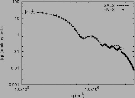
1:1, 1:2, 2:1 of samples A and B. The scattered intensity was measured
both with ENFS and a state-of-the-art SALS instrument. The data are
presented in Figs.
8.1,
8.2,
8.3,
8.4,
8.5
. Then, we
prepared three mixtures of them, respectively with volume fractions of
1:1, 1:2, 2:1 of samples A and B. The scattered intensity was measured
both with ENFS and a state-of-the-art SALS instrument. The data are
presented in Figs.
8.1,
8.2,
8.3,
8.4,
8.5
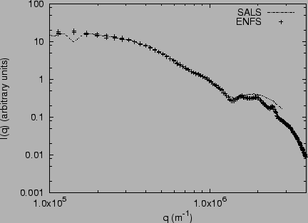
Figure:
Scattered light
intensity measurement of a
 colloid (sample A).
|
|
Figure:
Scattered
light intensity measurement of a
 colloid (sample B).
|
|
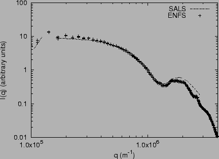
Figure 8.3:
Scattered light intensity
measurement of a mixture of the two samples. Volume fractions: 1/2 A,
1/2 B
|
|
Figure 8.4:
Scattered light intensity
measurement of a mixture of the two samples. Volume fractions: 1/3 A,
2/3 B
|
|
Figure 8.5:
Scattered light intensity
measurement of a mixture of the two samples. Volume fractions: 2/3 A,
1/3 B
|
|
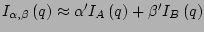
We define  and
and  the volume fractions of samples A and B
in each mixture; the scattered intensity of the mixture with a given
and is
the volume fractions of samples A and B
in each mixture; the scattered intensity of the mixture with a given
and is
 .
The scattered intensities
,
obtained for the three mixtures, are compared with
the scattered intensities
.
The scattered intensities
,
obtained for the three mixtures, are compared with
the scattered intensities
 and
and
 of the
two samples A and B. We evaluate the values of
of the
two samples A and B. We evaluate the values of  and
and  for which
 , by looking for the minima
of the mean square deviation:
, by looking for the minima
of the mean square deviation:
![$\displaystyle \left\{ \begin{array}{l} \alpha'=\frac { \sum_q{I_{\alpha,\beta}\...
...left[\sum_q{I_A\left(q\right)I_B\left(q\right) }\right]^2 } \end{array} \right.$](img508.png) |
(8.1) |
The values of and are the measured colloid concentrations,
and must be compared with and .
Table 8.1 shows the measured values,
and , compared with the actual ones, and .
Table 8.1:
Measured and actual values of volume concentrations of colloid A and B
in the three mixtures.
|
|
The agreement is
quite good: this shows that ENFS is suited for particle sizing.
The scattering data has been analyzed by an inversion algorithm based
on Mie theory. Mie theory allows to evaluate the scattered intensity
generated by
a given diameter distribution
 of dielectric spheres; the inversion
algorithm looks for the distribution
which
gives the best approximation to the measured
.
The results are shown in
Figs. 8.6 and
8.7.
Two peaks are quite
evident: they are centered on the diameters of
of dielectric spheres; the inversion
algorithm looks for the distribution
which
gives the best approximation to the measured
.
The results are shown in
Figs. 8.6 and
8.7.
Two peaks are quite
evident: they are centered on the diameters of  and
and  . The small peak centered around
 in the histogram
of Sample A corresponds to the scattering of the dymers: the colloid
is partially aggregated. The height of the peaks in
Fig. 8.7 change
accordingly to the fraction of the samples A and B in the mixture.
in the histogram
of Sample A corresponds to the scattering of the dymers: the colloid
is partially aggregated. The height of the peaks in
Fig. 8.7 change
accordingly to the fraction of the samples A and B in the mixture.
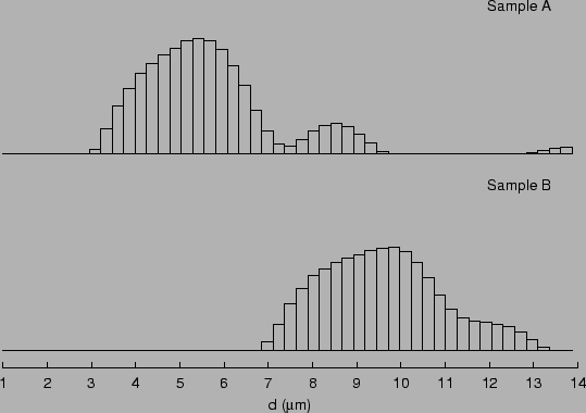
Figure 8.6:
Diameter distribution of the two colloidal samples measured by ENFS, obtained
by an inversion algorithm based on Mie theory. The height of the bars
is proportional to the intensity of light scattered by the particles
in the range covered by the horizontal extension of the bar.
Sample A is a
colloid, and sample B is a
 colloid. The two peaks are evident. Sample A shows
a small peak centered around
: it corresponds to the
scattering of the dymers.
colloid. The two peaks are evident. Sample A shows
a small peak centered around
: it corresponds to the
scattering of the dymers.
|
|
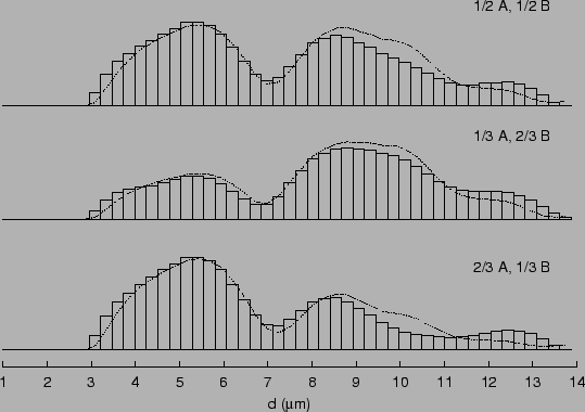
Figure 8.7:
Diameter distribution of the mixtures of colloidal samples, measured
by ENFS, obtained
by an inversion algorithm based on Mie theory. The height of the bars
is proportional to the intensity of light scattered by the particles
in the range covered by the horizontal extension of the bar. The
dotted curves are obtained by combining the values measured for samples
A and B, shown in Fig. 8.6
with coefficients given by the volume fractions of the two samples.
|
|
It should be noticed that ENFS measures the intensity of the scattered
beams with reference to the main beam. This allows to evaluate the
particle concentration, and not only the relative concentration of
different particles. This is accomplished by using a single sensor; on
the contrary, with SALS, the transmitted and the scattered beams must
be measured by independent sensors,
because the intensities are generally extremely different. This
difference comes from the fact that SALS sensors measure the intensity
of scattered beams, while ENFS measures the interference of them. For
example, consider a sample that generates a single scattered beam,
whose intensity is  than the transmitted one. For SALS, we
need two sensors, one for measuring the scattered beam and one for the
transmitted beam, and they require an accurate calibration. A single
sensor could be used without calibration, but its dynamic range should
cover 4 decades, and in this range it should be quite linear. For
ENFS, the interference of the two beams generates a modulation of
about
than the transmitted one. For SALS, we
need two sensors, one for measuring the scattered beam and one for the
transmitted beam, and they require an accurate calibration. A single
sensor could be used without calibration, but its dynamic range should
cover 4 decades, and in this range it should be quite linear. For
ENFS, the interference of the two beams generates a modulation of
about  . A single CCD array can easily measure such a
modulation.
. A single CCD array can easily measure such a
modulation.
Next: Non-equilibrium fluctuations in a
Up: Near Field Speckles
Previous: What is the main
Contents
2003-01-09