The intensity of the light scattered from a spatially disordered sample has a speckled appearance, the speckles being generated by the random interference of the scattered elementary spherical waves. While the study of the one point intensity time correlations has proven very useful, and it has generated the technique of Intensity Fluctuation Spectroscopy (IFS) [5], the measurement of the two point, equal time, intensity space correlation function, that is the size and the shape of the speckles, does not provide any useful information. Indeed the Van Cittert and Zernike theorem states that the far field space correlation function depends only on the intensity distribution of the scattering volume, and in no way depends on the physical properties of the sample.
In this chapter we will present qualitative elements showing that for fluctuations the size of the wavelength of light or larger, in the near field we obtain a speckle field, that is, a gaussian field; moreover its statistics is directly related to the scattered intensity distribution. We will derive the working formulas for three tecniques, hOmodyne Near Field Speckles (ONFS), hEterodyne NFS (ENFS) and Schlieren-like NFS (SNFS); analogies with the IFS will be pointed out. Advantages with respect to the more conventional Small Angle Light Scattering (SALS) technique will be discussed.
First of all, we will describe ONFS setup; many considerations hold also for ENFS and SNFS. The experimental set-up is very unorthodox, with respect to a conventional SALS device. It consists of a wide laser beam and of a Charge Coupled Device (CCD) detector positioned so to be flooded with light coming from any scattering direction the system can scatter at.
The Van Cittert and Zernike theorem states that the field correlation function is [6]:
where
![]() is
the field in the observation plane
is
the field in the observation plane ![]() ,
, ![]() is the
wavelength and
is the
wavelength and
![]() is the actual intensity
distribution of the source in the plane
is the actual intensity
distribution of the source in the plane
![]() at a distance
at a distance
![]() from the observation plane. The theorem holds for sources
consisting of point emitters, like atoms. The intensity
correlation function
from the observation plane. The theorem holds for sources
consisting of point emitters, like atoms. The intensity
correlation function
![]() is
then derived by applying the so called Siegert relation
[7]:
is
then derived by applying the so called Siegert relation
[7]:
Equations (2.1) and (2.2) specify that the intensity
correlation function is related to the space Fourier transform of
the source. In practice, this implies that a source of size ![]() will generate speckles of size
will generate speckles of size
![]() on a screen
positioned at a distance
on a screen
positioned at a distance ![]() [7].
[7].
We will start introducing simple euristic arguments and crude
evaluations for the near field speckles of the scattered light.
Let us consider the case of a large beam diameter ![]() ,
impinging onto a sample of particles of diameter
,
impinging onto a sample of particles of diameter ![]() larger than
the wavelength of light: see Figure 2.1(a). Most of
the power will be
scattered in a forward lobe of angular width
larger than
the wavelength of light: see Figure 2.1(a). Most of
the power will be
scattered in a forward lobe of angular width
![]() .
.
![\begin{figure}\begin{tabular}{cc}
(a)&
\parbox[c]{10cm}{
\begin{picture}(250,200...
...h(70,92)(70,104)(74,108)(74,96)(70,92)
\end{picture}}
\end{tabular}
\end{figure}](img29.png) |
Notice that all the above applies under conditions that are
more stringent than the usual ``near field'' condition [8]
for a source of size ![]() , namely
, namely
![]() .
In the present case the condition is
.
In the present case the condition is ![]() which implies
which implies
![]() .
.
To put things in a more quantitative way, we will determine the
near field intensity correlation by first re-writing the Van Cittert and
Zernike
theorem in a more appropriate form. We notice that Eq. (2.1)
may be rewritten in the following way:
Equation (2.3) is only a different way of writing Eq. (2.1), and
![]() is the intensity distribution of the source as seen
from the observation plane as a function of the scaled angles
is the intensity distribution of the source as seen
from the observation plane as a function of the scaled angles
![]() , and
, and
![]() .
As discussed in the introductory
remarks, in the very near field
.
As discussed in the introductory
remarks, in the very near field
![]() equals the
scattered intensity distribution, which is proportional to the Fourier
transform of
the sample density correlation function
equals the
scattered intensity distribution, which is proportional to the Fourier
transform of
the sample density correlation function
![]() , where
, where ![]() is the local
fluctuation of the particle number density, integrated over the light
path. Then, from Eq. (2.2), it follows that:
is the local
fluctuation of the particle number density, integrated over the light
path. Then, from Eq. (2.2), it follows that:
To determine the spatial intensity correlation of Eq. (2.4), one
must first obtain experimentally the instantaneous intensity
distribution of the near field scattered light. In order to
evaluate the intensity correlation function with reasonable
statistical accuracy it is also imperative to gather intensity
distributions over a substantial number of points. To this end a
CCD is ideal, the number of pixel being larger than ![]() . As we
shall see, it actually turns out that one frame is enough for a
fair acquisition of the correlation function.
. As we
shall see, it actually turns out that one frame is enough for a
fair acquisition of the correlation function.
In a previous work [1],
some measurements have been performed on a scattering model, an opaque
metallic screens with pinholes of 140 and 300 microns chemically
etched in random positions. The surface fraction occupied by the
pinholes was around 10% and 20% respectively. Experimentally this
greatly simplifies the problem, since the scattered field is
stationary and also there is no transmitted beam.
We call this configuration hOmodyne Near Field Speckles, since the signal
is given by the interference of different scattered beams.
Being a two
dimensional sample, the scattered intensity was simply related to
the correlation function of the transparency function
![]() with
with ![]() inside the pinholes and zero outside [6]. A
Helium Neon parallel beam with diameter (
inside the pinholes and zero outside [6]. A
Helium Neon parallel beam with diameter (
![]() points)
points)
![]() was sent onto the samples, and the speckle field was
recorded with a CCD at various distances
was sent onto the samples, and the speckle field was
recorded with a CCD at various distances
![]() ,
,
![]() and
and
![]() 2.1.
The corresponding values for
2.1.
The corresponding values for ![]() ranged
from
ranged
from
![]() to
to
![]() so that the very near field condition was
always met. The rather large dimension of the pinholes was chosen
so that the speckles were appreciably larger than the CCD pixel
size (typically
so that the very near field condition was
always met. The rather large dimension of the pinholes was chosen
so that the speckles were appreciably larger than the CCD pixel
size (typically
![]() ). For each type of pinholes, the
measurements performed at the three distances showed minute
differences. The results are shown in Fig 2.2, where
the data
are compared with the correlation functions of digitised images of
the set of pinholes on the metallic screen
2.2.
Since in this case the sample is two-dimensional,
). For each type of pinholes, the
measurements performed at the three distances showed minute
differences. The results are shown in Fig 2.2, where
the data
are compared with the correlation functions of digitised images of
the set of pinholes on the metallic screen
2.2.
Since in this case the sample is two-dimensional,
![]() is the correlation function of
is the correlation function of
![]() .
.
![\includegraphics[scale=0.5]{giglio2.eps}](img68.png) |
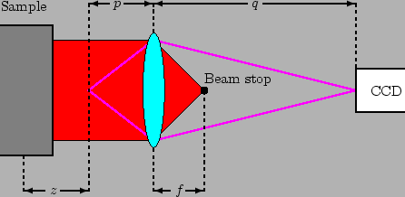
While the data obtained with the screens prove that near field speckles do mirror the properties of the scatterers, we feel that to assess the desirability of the technique for realistic applications (for example in colloid physics) measurements had to be taken with particle solutions down in the micron range. In order to do this, three problems had to be solved. The speckles in the near field close to the cell have dimensions around one micron and therefore are too small for the available CCD pixel size. Also, one must dispose of the transmitted beam. Finally, the speckle intensity distribution must be frozen at a given instant.
The first two problems have been solved with the simple optical arrangement shown in Fig. 2.3.
 |
When the scattered speckles
are observed with the CCD in real time, one notices quite vividly
that the speckle size changes as the size of the scatterers is
changed. Also, for a given sample the speckles boil with the
same time constant on the whole screen, the time constant getting
larger for samples with larger diameter particles. With regard to
the third problem mentioned above, these observations also
indicate that even with a conventional CCD and a small power He-Ne
laser there is no problem in getting instantaneous pattern
distributions. Indeed even for the smallest particles that can be
studied with present experimental set-up, with diameters
down to
![]() , and
assuming diffusive motion, the shortest time constant associated
to the smallest scattering wavevector yields
, and
assuming diffusive motion, the shortest time constant associated
to the smallest scattering wavevector yields
![]() ,
a time long compared with the shortest frame exposure
available with standard frame grabbers, typically
,
a time long compared with the shortest frame exposure
available with standard frame grabbers, typically
![]() .
.
Let us compare the Near Field Speckles technique with the more traditional
Small Angle Light Scattering. The essential feature of a scattering layout
[11,12] is that the light scattered at a given angle
hits the sensors along a circle of given diameter around the
optical axis. We believe that the correlation method of NFS offers some
distinct advantages over the scattering technique. First, there is
no need for accurate positioning of the CCD, that can be rather
casually placed at a distance ![]() from the focal plane (see Fig.
2.3). At variance, in SALS one has to know
the precise relation between pixels and scattering angles and this
is troublesome when the distance
from the focal plane (see Fig.
2.3). At variance, in SALS one has to know
the precise relation between pixels and scattering angles and this
is troublesome when the distance ![]() is changed to select a new
particle diameter instrumental range. Also, and more important,
SALS is plagued by stray light. To mitigate its
effects, one has to rely on blank measurements to be subtracted
from raw scattering data. The trouble is that stray light is worst
at smaller angles, where the sensing elements are necessarily in
small number and crowded close to the optical axis. With the
present technique, on the contrary, all the pixels are used in
calculating the correlation function for any value of the
displacement
is changed to select a new
particle diameter instrumental range. Also, and more important,
SALS is plagued by stray light. To mitigate its
effects, one has to rely on blank measurements to be subtracted
from raw scattering data. The trouble is that stray light is worst
at smaller angles, where the sensing elements are necessarily in
small number and crowded close to the optical axis. With the
present technique, on the contrary, all the pixels are used in
calculating the correlation function for any value of the
displacement ![]() and this allows more accurate stray light
subtraction; the algorithms to subtract the stray light will be described
in Chapter 5.
and this allows more accurate stray light
subtraction; the algorithms to subtract the stray light will be described
in Chapter 5.
The results of the measurements on some colloid samples are presented in Chapter 7. The ONFS technique in the present form has only one tight requirement, namely the clean disposal of the transmitted beam that requires accurate focusing and a proper diffraction limited beam stop. It is both conceptually and in practice very simple, and it capitalizes on the high statistical accuracy permitted by the large number of pixels of a CCD and by the good handling capabilities of PCs.
It became soon appearent that the main problem with ONFS comes from
the poor statistical quality of the calculated
![]() .
In Chapter 7 we
will show that the statistical quality increases only as the fourth
root of the number of processed images. We experimented a different
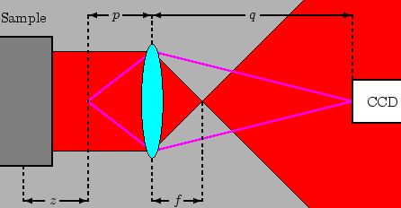
optical setup (ENFS), drawn in Fig. 2.4.
.
In Chapter 7 we
will show that the statistical quality increases only as the fourth
root of the number of processed images. We experimented a different
optical setup (ENFS), drawn in Fig. 2.4.
 |
Basically, ONFS data processing consists in evaluating the field
correlation function
![]() by using Siegert
relation (2.2), then evaluating
by using Siegert
relation (2.2), then evaluating
![]() by applying
the inverse Fourier transform to
(2.3). In ENFS, we measure the interference between the speckle
field of ONFS with the much more intense transmitted beam. We directly
measure a quantity linearly related to the field. The intensity
correlation function of an ENFS image equals
by applying
the inverse Fourier transform to
(2.3). In ENFS, we measure the interference between the speckle
field of ONFS with the much more intense transmitted beam. We directly
measure a quantity linearly related to the field. The intensity
correlation function of an ENFS image equals
![]() , provided that all the conditions needed by ONFS
are met, that is, if the field is circular gaussian. We thus obtain
, provided that all the conditions needed by ONFS
are met, that is, if the field is circular gaussian. We thus obtain
![]() without the data inversion needed to apply
Siegert relation, and this greatly enhances the statistical accuracy of
the results.
without the data inversion needed to apply
Siegert relation, and this greatly enhances the statistical accuracy of
the results.
In Chapter 7 we show a comparison between data taken with ONFS and ENFS; data taken with ENFS are evidently much less noisy. The quality is comparable with the SALS one. This good quality allowed to try a Mie-based inversion algorithm, to obtain an histogram of the distribution of the diameters of some colloidal samples; the measurements are shown in Chapter 8.
Both ONFS and ENFS are quite sample wasting techniques. They require
a sample much bigger than the statistical quality needs. For
example, consider a non-equilibrium fluctuation measurement in a free
diffusion experiment [13]. The biggest fluctuations we want to
measure are
about
![]() . A good statistical sample should be so big to contain
some hundred of the biggest fluctuations: it can be a square with a
. A good statistical sample should be so big to contain
some hundred of the biggest fluctuations: it can be a square with a
![]() side. This is enough for SALS, but not for ONFS nor ENFS.
In Chapt. 3 we will show that, if we
want to cover two decades in wavevectors, we must use a sample with
side
side. This is enough for SALS, but not for ONFS nor ENFS.
In Chapt. 3 we will show that, if we
want to cover two decades in wavevectors, we must use a sample with
side
![]() . To cover two decades, we need a
half a meter wide
cell, while with SALS we can work with a half a centimeter wide cell!
This is not a difficulty for particle sizing applications, but can
become a serious problem when we want to analyze many
lenghtscales, since NFS is particularly suited for big objects.
This problem is essentially due to the fact that big objects need long
values of
. To cover two decades, we need a
half a meter wide
cell, while with SALS we can work with a half a centimeter wide cell!
This is not a difficulty for particle sizing applications, but can
become a serious problem when we want to analyze many
lenghtscales, since NFS is particularly suited for big objects.
This problem is essentially due to the fact that big objects need long
values of ![]() in order that their scattered field is gaussian; on the
other hand, we need a big sample, so that the sensor collect the light
scattered at high
angles by small particles. This fact is quite unusual, since in
general big objects are good subjects for classical microscopy
techniques.
The difficulty can be easily circumvented, introducing a new instrumental
setup, called SNFS: see Fig. 2.5.
in order that their scattered field is gaussian; on the
other hand, we need a big sample, so that the sensor collect the light
scattered at high
angles by small particles. This fact is quite unusual, since in
general big objects are good subjects for classical microscopy
techniques.
The difficulty can be easily circumvented, introducing a new instrumental
setup, called SNFS: see Fig. 2.5.
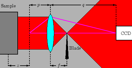 |
SNFS requires an additional element with respect to ENFS, the blade, but it allows easy measurements on many lengthscales, on big objects. We used such a technique to measure the power spectrum of non-equilibrium fluctuations in a free diffusion experiment, described in Chapter 9, thus showing that this technique can be applied to researches in fundamental physics.
![$\displaystyle C_E (\Delta x, \Delta y) = \left< E \left(x,y\right)
E^*(x+\Delta...
...i}{\lambda z} \left( \xi \Delta x +
\eta \Delta y \right) \right] d \xi d \eta}$](img13.png)
![$\displaystyle C_I\left(r\right) = \left< I\right>^2\left[1 + \left\vert\int{I\left(q\right)
e^{i\vec{q} \cdot \vec{r} }\mathrm{d}\vec{q}}
\right\vert^2 \right] .$](img50.png)