| Lab 1 of 40A| Main Menu Page| Lab 3 of 40A|

Introduction

On page 10, y=(1/2)gt² where y is the falling distance measured from the highest (or rest) point, and t is the time starting from the instant that the ball is released.

When we make a table of falling times, we will use d instead of y to represent the falling distance. However, they two are exactly the same.

Procedure

Step 2-4

Measure the distance d from the bottom of the ball to the receptor plate.

Step 2-6

Do not press until you finish a series of measurement with the same falling distance. Or your measured time will be erased from your computer.

After finishing a series of falling times, a data table will be shown on you screen. The Row of "Mean" stands for t_awg on page 13. And we do not need to record any error at this stage.

Step 2-10

Complete the given tables in the outline. Refer to Page 13.

Print no data table out during Lab 2. It is enough to fill your data in the given data table.

Step 3

Calculate t _average (1 point) and D t_RMS (1 point) with only one sample calculation. The others in Step 3 are optional.

Outline for "Acceleration of Gravity", 10/11/1999

1. Experiment title/ date
2. Your Name, Your E-mail Address (if applicable), Your Partner, and Section No.
3. Concept

1. State of purpose or theory regarding this experiment you like to write down
2. Basic formulas used

1. Measurements and Analysis

1. Measurements of necessary constants

Object	Weight, Unit : (    )	Diameter, Unit: (    )
Small ball
Big ball

2. Measurements of gravity, g, for the small ball, referring to Page 17:

(y-y0), Unit: (    )	Five elapsed time, Unit:(    )					t average (    )	D tRMS (    )
	t1	t2	t3	t4	t5

Calculate t _average (1 point) and D t_RMS (1 point) with only one sample calculation.

3. Results of Analysis, for the small ball:

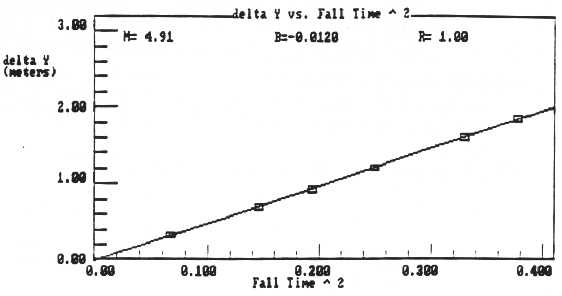
Plot "y-y₀ vs. t" graph on screen. Modify “t _average” to get Graph "d versus t _average ²." (0.5 point)

Print out the modified graph with “statistics” for modified data and find out "g _fitted".

Calculate %error: g _true = 9.795 m/s² , σ_g = standard deviation of slope

(0.5 point) [(g _fitted - g _true) / g _true] ´ 100%=

(0.5 point) (2σ_g / g _fitted ) ´ 100%=

4. Do "2" and "3" again for the big ball. For your "(y-y₀) vs. t_average²", Accuracy, and Precision, each, 0.5 point is.

5. This additional part regarding "air resistance" is for the questions and the remarks on page 15.

	g average, Unit:(    )	A/m, Unit:(    )
Small ball
Big ball

Plot and print "g_average vs. A/m."

"A" is the shadow area of the body projected on a horizontal plane. For a ball, A=p R².

This is a Sample Graph for your practice only.



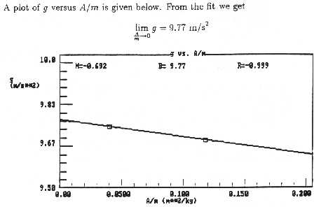
"m" is the mass of the ball.

You have only two data points for this graph, which are associated with two balls.

Additional Question 1, Comparison, 1 point

Consider that the magnitude of air resistance is proportional to "A/m". Based on "g_average vs. A/m", we have an empirical relation between g _average and A/m. Please write it down as Y= [M]X + [B] and plug in the values of [M] and [B] you have.

Additional Question 2, Errors, 1 point

Here is a follow-up. Define that [%error]_g = |[( g _average - g _true) / g _true] ´ 100%|. Now, let's say that the reasonable percentage error of g _average is [%error]_g <1%, or -1%< [(g _average - g _true) / g _true] ´ 100%] <1%. What are the upper and lower bound of “A/m” to get the reasonable percentage error of g _average ?

In other words, if “A₁/m₁”<“A/m”<“A₂/m₂”, what are your numerical values of “A₁/m₁” (0.5 point) and “A₂/m₂” (0.5 point) when [%error]_g <1%?

Question 3, Application of Graph “g _average versus A/m”, 1 point

It is on Page 12. “From g values measured with two different size balls, can the measured g be extrapolated to A/m=0?” It will be easier, at first, to figure out the physical situation of a ball as “A/m” goes to 0.

2. Conclusions

Answer all three additional questions.

3. Suggestion

| Lab 1 of 40A| Main Menu Page| Lab 3 of 40A|