| Main Menu Page| Lab 2 of 40A|
Lab 1, Computer Aided Measurements,
10/04/1999Courtesy of Chiung-Yuan Lin
| DATA TABLE - "MOTION TIMER" Mode | |
|
ROW # |
TIME (sec.) |
|
1 |
0.0403 |
|
2 |
0.0314 |
|
3 |
0.0266 |
|
4 |
0.0236 |
|
5 |
0.0214 |
|
6 |
0.0195 |
|
7 |
0.0185 |
|
STATISTICS: |
|
|
#: |
7 |
|
MEAN: |
0.0259 |
|
SD: |
0.0077 |
|
SDOM: |
0.0029 |
|
MIN: |
0.0185 |
|
MAX: |
0.0403 |
Procedure I- Computer Aided Measurements, v versus t:
Step 4
Please practice dropping the picket fence. Hold it gently by one end, and release it smoothly so that it falls straight. All of the bars on the fence should interrupt the photo-gate.
Step 5
A typical set of data will look, on your computer screen, like this:
This sample data table is only for your reference and not needed in your report.
Step 7
Use measurement of strip spacing d from step 1.
Step 10
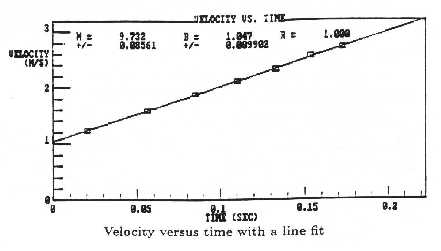
The graph of velocity versus time should present you a straight line, a regression line, with a positive slope. From the sample data table given in Step 5, we will have a constant, slope[M].
Here, slope [M] = g =9.732± 0.086(m/sec2).
Step 11
Whenever you printout something, after you selected the "print" option, you should wait at least one minute before you hit the printout key again. It is to avoid the data-bus jamming in the laser printer and to save your time.
Step 12
As to the degree of agreement, follow the rule below.
Percentage error = c%.
Write c= a´< 10b with 1£< |a| <10.
The degree of c, cdeg will be:
cdeg = 10b%, if |a| <10(1/2),
cdeg = 10b+1%, if |a| >10(1/2), where 10(1/2) »< 3.16227766
Therefore, you can compare cdeg between different errors.
For example, using the sample value g obtained from Sample Data Table in Step 5 and referring to the equations on page 7, we have:
Accuracy:A, (gmeasured-gtrue)/gtrue ´< 100% = (9.732-9.80)/9.80´< 100% = -0.7%= -(7´< 10-1)%
cdeg = 10(-1+1) %= 1%
Precision:B, (+/-)error/ gmeasured ´< 100% = 0.086/9.732´< 100% = 0.88%= (8.8´< 10-1)%
cdeg = 10(-1+1) %= 1%
The degrees of two percentage errors are the same, obviously.
The sign "-" of the first error from Equation A means that gmeasured is below gtrue.
Remark:
Notice that 0.086/9.732´< 100% = 0.9% but 0.086/9.732´< 100 ¹< 0.9%!
This kind of mistakes will cost you 0.5 points, every time, consecutively!
Question 12-1 on page 7.
Calculate the percentage error of your measurement two ways, using gtrue = 9.80(m/sec2)
Requirement: Use equations A (0.5 Point) and B (0.5 Point). Put your first gmeasured, g1 in the two equations and show your work.
Question 12-2 on page 7.
Discuss briefly the degree of agreement of these two percentage errors.
Requirement: (0.5 Point) Make your judgement with logical reasons. (0.5 Point) Answer them in percentage.
Step 13
Repeating this measurement five times gives the sample table of values below.
| Gravity |
g± d g, (m/s2) |
|
g1 |
9.732± 0.086 |
|
g2 |
9.753± 0.068 |
|
g3 |
9.918± 0.120 |
|
g4 |
9.826± 0.098 |
|
g5 |
9.778± 0.098 |
From this Sample Data Table, using gi without errors, we can calculate the mean value of g, gave, and the Standard Deviation of g, D gRMS. Here, RMS means Root-Mean-Square.
gave = (g1+g2+g3+g4+g5)/5 = 9.8014(m/sec2)
D gRMS = {[(g12+g22+g32+g42+g52)/5]- gave 2}(1/2) = 0.066(m/sec2)
(D gRMS / gave) = 0.066/9.8014´< 100% = 0.7%
Here, cdeg = 10(-1+1) %= 1%, the degree of the RMS spread in g values is the same as the two errors estimated from Step 12.
Notice the calculation of D gRMS is very sensitive to how many digits you keep during the intermediate steps. So, during your intermediate steps, keep as many digits as possible.
Remark:
Notice that 0.066/9.8014´< 100% = 0.7% but 0.066/9.8014´< 100 ¹< 0.7%!
This kind of mistakes will cost you 0.5 points, every time, consecutively!
Question 13-1 on page 7.
Compare the variation of g values from the measurement with your own error estimate from Step 12.
Requirement: (0.5 points) Write down your true value of g at first. Then make your judgement with logical reasons. (0.5 points) You must answer it in percentage.
Procedure II- Graphical Analysis on the IBM:
Part A. Getting Started with Graphical Analysis on the IBM:
Step 3
Use Sample Data Sets 8 on page 13.
Step 5
You do not have to print out one copy of your selected data table, but if you do, please tape it nicely into your notebook.
Part B, Displaying the Graph:
Step 5
Print out one copy of your unmodified graph of Set 8, and tape it nicely into your notebook.
Part C, Modifying the Graph:
Step 1
Here are three examples to modify Sample Data Sets 2-4.
For Set 2, we have t=ch0.5. Comparing it with the slope on your modified graph “t versus h0.5”, you will find that c = (slope [M]) and t= (slope [M])´< h0.5.
For Set 3, treat your graph “y versus x” as the modified graph “t versus d-1”, you will find that c = (slope [M]) and t= (slope [M])´ d-1.
For Set 4, Comparing ln(T)= ln(K)+n´< ln(d ) with the slope [M] and Intercept [B] on your modified graph “ln(T) versus ln(d )”, you will find that n= (slope [M]) and ln(K)= (Intercept [B]).
Therefore, you have n= (slope [M]) and K= e(Intercept [B]). We trace back to the original equation, T=Kdn and find T= e(Intercept [B])´ d(slope [M]).
Step 2
You do not have to print the modified data table. Only one modified graph is required.
Part D, Best-fit Straight-line Parameters.
You have to understand Part D in your lab manual clearly and answer the following question. Then skip the requirements of this part on page 10.
<
Alternative Question D-3-1:Compare your two graphs before and after modification. Write down the difference among them regarding the data points, the regression line, and the correlation coefficient [R]. Of course, you must answer them all in percentage. Also, write down the qualitative difference between the graphs before and after modification.
Procedure III- Outline of Lab Notebook Contents (This experiment only)
It may not be given every week.
A, Date and Title of Each Experiment
B, Your Name, Your E-mail Address (if applicable), Your Partner, and Section No.
Procedure I, Computer Aided Measurements
1. State of Purpose.
2. Relevant formula(s).
3. Measurement of picket fence spacing, d.
4. Your graph v versus t.
5. Your data table of gravity, g, with error.
6. Percentage errors with questions 12-1, 12-2, and 13-1 on page 7.
Procedure II, Graphical Analysis
1. State of Purpose.
2. Print out your selected data table in Step 5, Part A.
3. Relevant formula(s).
4. Your graph of data selected before modification.
5. Your graph of data selected after modification.
6. Values of slope [M] and intercept [B].
7. Answer Alternative Question D-3-1.
-----------Detach it, please-----------
Suggestion
| Main Menu Page| Lab 2 of 40A|
My Home Page