Intended Learning Outcomes
At the end of this section students should be able to complete the following tasks.
- Describe the structure of back-propagation and SOM neural networks.
- Outline the effects that the design decisions have on the potential performance of a neural network.
- Use a weight interpretation algorithm to identify the relative importance of predictors to a back-propagation neural network.
- Decide whether a neural network is more sutiable than a generalised linear model for an application.
Background
During the early years of Artificial Intelligence (AI) research it was thought that machines could be built to simulate intelligent behaviour. During this time the two main AI branches were lead by Minsky and Rosenblatt. Minsky was concerned with a symbolic, rule-based approach to AI that is now linked to Expert Systems and programming languages such as LISP and Prolog while Rosenblatt favoured a connectionist approach to AI that was based on a simplified biological neural network and reflected his early career as a psychologist. Despite an early scare, the connectionist approach was rejuvenated in the 1980s, particularly following the publication of McClelland and Rumelhart's (1986) influential 'Parallel Distributed Processing' book.
Artificial neural networks belong to the class of methods that are variously known as parallel distributed processing or connectionist techniques. Although they attempt to simulate a real neural network, most artificial neural networks are simulated since they are implemented in software on a single CPU, rather than one CPU per neurone.
Neural networks tend to perform well when data structures are not well understood. This is because they combine and transform raw data without any user input (Hand and Henley, 1997). Thus they can be particularly useful when a problem is poorly understood. If there is considerable background knowledge, including knowledge of probability density distributions, it is usually better to use methods that incorporate this information (Hand and Henley, 1997). In general, neural networks perform well when the main requirement is for a 'black box' classifier rather than a classifier that provides insight into the nature of class differences.
Despite their early promise neural networks have not fully delivered what was originally expected, possibly because the expectations were too high and they seem to have been used inappropriately in many studies (see Schwarzer et al (2000) for detailed examples). Many artificial neural network applications do little more than replicate standard statistical methods, but with the added complication of a lack of transparency.
The following pages provide only a brief outline of two network architectures: back- propagation (multilayer perceptron) and SOMs (self-organising maps). There are many other useful network architectures, such as radial bias functions, that are not described here. The following six sources are recommended for more information.
- Ripley's (1996) "Pattern Recognition and Neural Networks".
- Boddy and Morris (1999) describe, amongst others, the background to multilayer perceptrons and radial bias function networks, set within the context of automated species identification.
- Cheng and Titterington (1994) and Sarle (1994) review the links between neural networks and statistical methods.
- Goodman and Harrell (2001a,b) are very useful descriptions of multilayer perceptrons and their links to generalized linear modelling. The background to multilayer perceptrons is set in the context of their very powerful and free NEVPROP neural network software (Goodman, 1996) that is used elsewhere in this section.
- The neural network FAQ at ftp://ftp.sas.com/pub/neural/FAQ.html. These FAQs were last updated in 2000.
Back-propagation
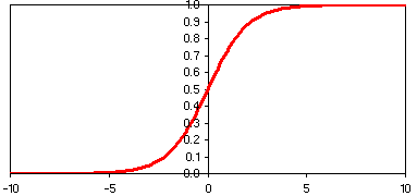
An artificial neural network is composed of a simple processing elements called nodes or neurons. Nodes convert the inputs to an output between 0 and 1. The conversion passes a weighted sum of the inputs, via a transfer function, to the output. Transfer functions, such as the logistic function 1/(1 + e-input), are typically sigmoidal (see below). The value passed to the transfer function is wi.pi + constant. In neural network terminology the constant is known as the bias.
The structure of a single node is summarised below. Despite its relative simplicity the single node is equivalent to the logistic generalized linear model.
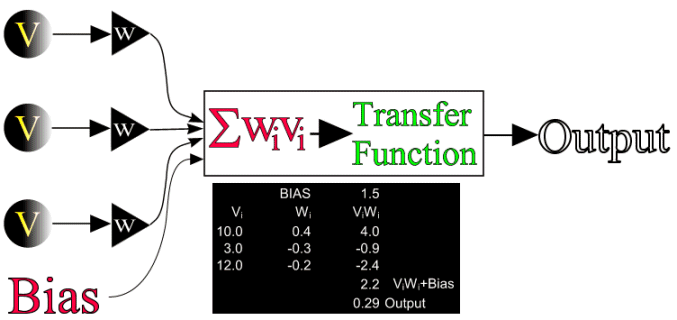
Io this simple example there are three inputs with values 10, 3 and 12 which pass through weights of 0.4, -0.3 and -0.2. The bias is 1.5 giving a sum of 4.0 + (-0.3) + (-0.2) + 1.5 = 2.2. If this value is passed to the logistic function the output from the node is 0.29.
Real neural networks have more than one node, which may be arranged in inter-connected layers. The number of inputs to the nodes is fixed by the number of predictors and the number of outputs is fixed by the number of classes. Only one output is required for two classes. Typical multi-layer perceptron neural networks have three layers: input; hidden (middle); and output.
1 |
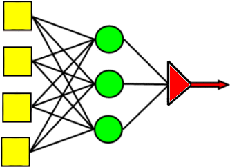
How many weights?The network above has two layers. The first layer (yellow squares) has four input nodes which are connected to a hidden layer of three nodes (green circles). The hidden layer is, in turn, connected to a single output node (red triangle). How many weights are there in this network? |
The network's model of the relationship between the predictors and the class (the output) is dispersed, or distributed, though its weights and this complexity should make it reasonably robust (e.g. tolerant of missing values). However, because the relationship is spread amongst the weights it can be difficult to interpret the relationship between the class and the predictors.
The network 'learns' the appropriate model by adjusting the weights to maximise the accuracy of the predictions given a set of training data. This is achieved via a series of iterative adjustments to the weights during a training phase. One of the most common algorithms used to implement this training is known as back-propagation although there are others such as the Levenberg-Marquardt algorithm and conjugate gradient descent.
At the start of training the network weights are randomised and there is no reason to believe that the network will perform better than guessing. The values from the predictor variables for the first case are passed to the network where they pass through the 15 weights and four transfer functions to produce an output in the range 0 - 1.
If there are two classes they would be represented by 0 and 1. Imposing a simple 0.5 threshold to the output means that a case will have a predicted class of 0 if the output is < 0.5 and 1 if the output is > 0.5. Most cases will not have outputs at the 0 and 1 extremes and the difference between the actual class and the output is a measure of network's current inaccuracy. Inaccurate predictions arise because the weights have the wrong values. The prediction error could be corrected by adjusting the weights.
The 'learning' takes place by deciding which weights to adjust. All weights will not contribute equally to the prediction error and it is reasonable to base the size of any adjustment on the size of the error. If the error is small only small weight adjustments are required. The back-propagation weight correction algorithm measures how the error is propagated back through the network's weights. After the weights have been adjusted the next case is applied to the network and the weight adjustment procedure is repeated. Once all of the cases in the training set have passed through the network one epoch has been completed.
A full training cycle could involve hundreds of epochs. A decision to stop training is made when pre-specified termination criterion is reached, for example a small enough error rate has been reached.
The adjustments to individual weights take account of the size of the output error and the magnitudes of the outputs from the nodes feeding directly, or indirectly, into the output node. It is reasonable to assume that nodes with the largest outputs make the largest contribution to the prediction error, in which case their weights should experience the largest adjustments. The full details of weight adjustment algorithms are not given here but they can be found in many online and printed sources, such as the artificial intelligence repository.
Deciding when to stop training is important because if a network is over-trained its future performance will be compromised. Usually, training is stopped by keeping track of the size of the training error that is measured as the sum of squared errors. In a statistical model there are well defined rules that guarantee to find the parameter values that minimise the error. However, because network training is heuristic the rules do not exist and judgement must be used. In order to avoid over-fitting some data are reserved for testing. If the network becomes over-trained the test error will begin to rise, even though the training error may still be declining. An increase in the testing error is an indication that training should stop. Ideally the network should experience a final test using a third set of data that played no part in the training.
Statistical models
Many neural networks differ very little from statistical techniques as evidenced by Goodman's description of his NevProp software as a multivariate non-linear regression program. Indeed the design of the network (e.g. how nodes are connected) can be used to duplicate specific statistical models. For example, the first network diagram (above) is effectively a generalized linear model in which each predictor is linked, by a single weight or coefficient, to the output node where a logistic transfer is applied to convert the weighted sum to an output within the range 0 to 1. If a neural network can also be a GLM, how do we decide when a neural network is appropriate? Firstly, Goodman and Harrell (2001a, b) emphasise that statistical approaches concentrate on the parameter values and their significance levels while neural networks, and other machine learning methods, are more concerned with prediction accuracy when presented with novel data. Secondly, they describe guidelines to decide if a neural network should be used in preference to a generalized linear model. These are summarised below.
- A neural network should only be used when the relationships between the class and predictors include non-linear relationships and between-predictor interactions.
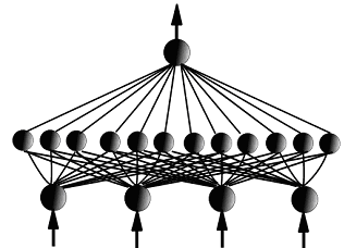
- A single hidden layer neural network, with fully connected links between the input nodes and
the hidden nodes, models, simultaneously, predictor transformations and interactions. The
complexity of these transformations and interactions is controlled by the size of the hidden
layer.
- Goodman and Harrell (2001 a, b) suggest comparing the results from a generalized model with those of a neural network with a single hidden layer. Even though they may be desirable, the generalized linear model should not include any interactions or predictor transformations. They suggest using AUC of a ROC plot and Nagelkerke's R2 to make the comparisons. If the network accuracy is not significantly better than the GLM there are two conclusions. Firstly, there is no point using a neural network. Secondly, and more usefully, there is no need to 'improve' the GLM by incorporating interactions or predictor transformations.
- The neural network would be more accurate only if interactions and/or transformations were missing from the statistical model.
- If all of the predictors were all binary the improvement must be due to interactions which could be identified and incorporated into the GLM.
- If some of the predictors were non-binary the improvements due to interactions and transformations have to be separated.
- A neural network can be designed that does not model interactions but can transform the
predictors automatically.
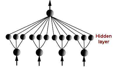
This 'transforming' network has a hidden layer in which groups of hidden nodes are connected to single predictors. These discrete clusters carry out transformations that are not pre-specified and can differ between predictors. Increasing the number of nodes in a cluster makes the transformations more complex in a similar way to the smoothing function in a generalized additive model. - If this interaction-free network performs as well as the original fully-connected network the improvement must be a consequence of transformations rather than interactions. If the appropriate transformations can be identified they could be included in statistical mode.
- If the transforming network is not as accurate as the original network it is worth considering using a neural network.
Although these comparisons may take some time Goodman and Harrell (2001 a, b) point out that using neural networks in this exploratory role avoids the need to spend time trying to refine a GLM when it is not needed or possibly too complex. It also provides a solid case for the use of a neural network.
Interpreting Weights
The interpretation of statistical models involves examining the values for the coefficients. It is not a simple matter to complete a similar assessment for neural networks. Neural networks are effectively black boxes, where the values for the coefficients are dispersed through the weights, spread across several nodes and layers. This is further complicated because the weights are not unique. They will alter if a network is trained with the cases in a different sequence or with different initial random weights. In other words, there are many weight combinations that may be equivalent to the fixed coefficients that would be estimated in a statistical analysis
Intrator and Intrator (2001) and Goodman (1996) describe methods that allow some interpretation of the contribution made by each predictor to the class. These methods assume that a predictor's generalized weights have the same interpretation as the coefficients in a logistic regression. The interpretations take account of the variability in the weights. A predictor that has a positive effect for some cases, and a negative effect for others, should have a mean effect of zero, but with a large variance. If the mean effect size is not zero then a small variance in the generalized weights suggests that a predictor's effect is consistent with a linear relationship, while a large variance is suggestive of a non-linear effect. The technical details for this approach are given in Intrator and Intrator (2001).
Olden et al (2004) carried out some empirical tests of a range of a range of weight interpretation algorithms on an artificial data set with a known structure. They compared how the different algorithms ranked the predictor importances across and how these ranks related to the real structure in the data. They concluded that the connection weight approach was the best. Fortunately this is also one of the simplest. A worked example is shown below.
The are five inputs (V1 to V5) which are fully connected to three nodes in a single hidden layer. The first part of the table shows the weights for these connections, for example the weight connecting V2 to hidden node 3 is 1.39. The three hidden nodes are connected to a single output node via a single weight, for example hidden node 2 has a connection weight of 1.57 to the output node.
| input | Hidden 1 | Hidden 2 | Hidden 3 | V1 | -0.63 | 2.14 | 0.44 | V2 | 0.50 | 2.57 | 1.39 | V3 | -1.32 | 0.54 | 0.38 | V4 | -1.30 | -0.68 | 0.23 | V5 | 1.65 | 0.14 | -1.89 |
|---|---|---|---|---|
| Hidden 1 | Hidden 2 | Hidden 3 | output | -1.21 | 1.57 | -0.95 |
| input | Hidden 1 | Hidden 2 | Hidden 3 | Row Sum | V1 | 0.76 | 3.36 | -0.42 | 3.70 | V2 | -0.61 | 4.03 | -1.32 | 2.11 | V3 | 1.60 | 0.85 | -0.36 | 2.08 | V4 | 1.57 | -1.07 | -0.22 | 0.29 | V5 | -2.00 | 0.22 | 1.80 | 0.02 |
The lower part of the table shows the products between the input-hidden and hidden-output weights. For example, the product of the weights between V4 and hidden node 1 and hidden node 1 to the output node is -1.30 x -1.21 = 1.57. The sum of the row products, for each predictor, are a measure of its importance. For example, the row sum for V1 is 0.76 + 3.36 + -0.42 = 3.70. Since this is the largest sum V1 is the is the most important predictor and V5 the least important.
Now examine the following weights and determine which is the most important predictor.
| input | Hidden 1 | Hidden 2 | A | -0.20 | 2.00 | B | 1.00 | 1.50 | C | -0.50 | 0.50 |
|---|---|---|
| Hidden 1 | Hidden 2 | output | -1.20 | 1.60 |
2 |
Weight interpretationThe weights above come from a network with three predictor variables: A, B and C. These three inputs are fully connected to a single hidden layer containing two nodes. The two hidden nodes are, in turn, connected to a single output node. Which of the following is the correct order of importance (most important first)? |
No detailed example analyis is presented because there are some very detailed examples in the NevProp manual. Even if you are not going to use this software it is still worth following through the details of the analysis.
Self-organising maps
Kohonen (1988, 1990) developed the Self-Organising-Map (SOM) algorithm to help with the problem of automated speech recognition. Software, and documentation, written by Kohonen and his collaborators can be downloaded from http://www.cis.hut.fi/research/som_pak/. Recently SOM networks have been quite widely used in the interpretation of gene expression profiles.
Although it uses an unsupervised learning method, that shares much in common with clustering methods, it is more generally referred to as an artificial neural network.
A SOM is a two-layered network:
- an input layer consisting of one node per variable
- each of the input nodes is connected to every node in the second, Kohonen, layer.
The size, and shape (rectangular or hexagonal), of the Kohonen layer, or grid, are design decisions. This grid is one of the important differences from most unsupervised clustering methods because it produces a solution in which similar clusters are close together.
There are weights connecting the input nodes to the Kohonen layer and, as in other neural networks, they are adjusted during training. The algorithm calculates how far, as a Euclidean distance, each Kohonen node's weights are from the input vector. The node whose weights are the closest match to the input vector (smallest distance) is identified as the winner and its weights are updated to increase the chance that the winning node will win again given the same input vector. Unlike other neural network algorithms, the weights of the winner's neighbours are also updated. The size and shape of the neighbourhood is another design decision but is typically Gaussian. The neighbourhood size is important because if it is too large small clusters may not be found and if it is too small large-scale patterns may not be captured. The size and shape of the neighbourhood allows weights to be updated by an amount that is related to a neighbour's distance from the winning node. Consequently, adjustments are smaller when distances are small. The size of the adjustment also depends on the size of the learning rate, which decreases gradually during training. As with the learning rate the neighbourhood size is gradually reduced during training.
SOM: Example analysis
This example uses the som function (version 0.3-4) from the R package to analyse some weather data collected by an automatic recoding station on the island of Mull (Hebrides) between August 1995 and August 1996. Data were collected every four hours, only data from 7 am to 5 pm are used in this analysis. The data are available on an Excel spreadsheet. There are seven variables: (1) total rainfall (mm in previous 4 hours); (2) Windspeed (4 hour mean) m / sec; (3) Wind direction (degrees); (4) Mean air temperature; (5) Relative humidity (%); (6) Solar radiation (kW / m2) and (7) Mean soil temperature at 10 cm.
The commands used to produce the analysis are outlined below.
First the data are loaded into a data frame from an SPSS file
som.data<-read.spss("mullweather.sav",to.data.frame=TRUE)
Next the variables are normalized to have a mean of zero and a standard deviation of one.
som.data.n<-normalize(som.data, byrow=F)
Now the SOM analysis is completed using a six by five grid with a rectangular topology
and a gaussian neighbourhood.
> weather.som <- som(som.data, xdim = 6, ydim =5, topol="rect", neigh="gaussian")
The results can be summarised by a plot (plot(weather.som)) which shows how the cases are spread between the thirty nodes in the Kohonen layer. The y-axis scale has standard normal deviate units and shows the mean values for the seven standardised variables.
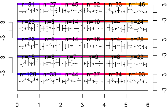
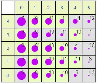
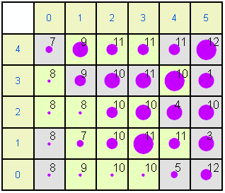
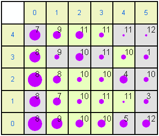
The same data can be shown in a more extended format. In each of the following plots the left and top rows show the node coordinates. The numbers within the other squares are the modal months. Some months are not represented because they do not achieve the highest frequency in any month. Gray nodes (such as 0,0) have 1995 as the modal year while pale green nodes (e.g. 0,1) have 1996 as the modal year. The size of circle is proportional to size of the mean for the variable. For example, in the rainfall map node 5,4 has a large mean (a lot of rainfall in December 1995) while node 0,0 has little rainfall in August 1995.
Rainfall
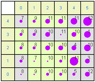
Wind speed
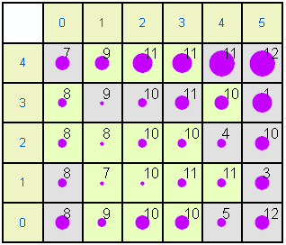
Air temperature
Relative humidity
Solar radiation
Soil temperature
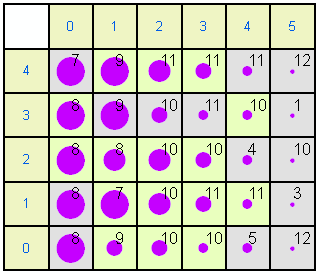
Examining the patterns in the Kohonen maps allows the different weather records to be categorised. There is an obvious Left - Right trend from Late Summer to Early/Mid winter. There is also a SW-NE humidity gradient.
Although the SOM algorithm does not suffer from the same problems as the hierarchical clustering algorithms there are still problems with identifying class boundaries. It is unwise to treat each grid in the Kohonen layer as a separate cluster. As can be seen above, clusters can be spread across several adjacent nodes. The difficulty is deciding which nodes should be grouped together to form clusters. The mechanisms that have been suggested to identify the class boundaries all involve some post-processing of the clustering results.

Resources
- Boddy, L. and Morris, C. W. 1999. Artificial neural networks for pattern recognition. pp 37-69 in A. H. Fielding (ed) Ecological Applications of Machine Learning Methods. Kluwer Academic, Boston, MA.
- Cheng, B. and Titterington, D. M. 1994. Neural networks: a review from a statistical perspective, Statistical Science, 9: 2-54.
- Goodman, P. H. 1996. NevProp software, version 3. Reno, NV: University of Nevada.
- Goodman, P. H. and Harrell, F. E. 2001a. Neural networks: advantages and limitations for biostatistical modeling. (pdf file).
- Goodman, P. H. and Harrell, F. E. 2001b. NevProp Manual with Introduction to Artificial Neural Network Theory (pdf file).
- Goodman, P. H. and Rosen, D. B. 2001. NevProp Artificial Neural Network Software with Cross-Validation and Bootstrapped Confidence Intervals.
- Hand, D. J. and Henley, W. E. 1997. Statistical classification methods in consumer credit scoring: a review. Journal of the Royal Statistical Society, Series A, 160: 523- 541.
- Intrator, O. and Intrator, N. 2001. Interpreting Neural-Network Results: A Simulation Study. Computational Statistics and Data Analysis 37(3): 373-393.
- Kohonen, T. 1988. An introduction to neural computing. Neural Networks, 1: 3 - 16.
- Kohonen, T. 1990. The self-organising map. Proceedings of IEEE, 78: 1464-1480.
- McClelland, J. L., Rumelhart D. E. and the PDP Research Group (editors). 1986. Parallel Distributed Processing. MIT, Cambridge, MA.
- Olden, J. D., Joy, M. K. and Death, R. G. 2004. An accurate comparison of methods for quantifying variable importance in artificial neural networks using simulated data. Ecological Modelling, 178: 389-397.
- Ripley, B. D. 1996. Pattern recognition and neural networks. Cambridge University Press, Cambridge.
- Schwarzer, G., Vach, W. and Schumacher, M. 2000. On the misuses of artificial neural networks for prognostic and diagnostic classification in oncology. Statistics in Medicine, 19: 541-561.
- Self-organizing maps Department of Computer Science and Engineering at the Helsinki University of Technology. http://www.cis.hut.fi/research/som-research/
Do not treat this list as comprehensive. If you discover another interesting site please let me know.

