
Intended Learning Outcomes
At the end of this section students should be able to complete the following tasks.
- Interpret the output from a binary logistic regression of a data file with continuous predictors.
- Identify those predictors that have a significant effect on the class of a case.
- Calculate confidence limits for a predictor's coefficient.
- Use diagnostic statistics to identify possible problems with an analysis.
- Explain the term deviance.
- Assess the value of the analysis from the accuracy and the diagnostic statistics.
The data
Data set B (available as an Excel file or a plain text file) has four continuous predictors (b1 to b4) and two
classes with 75 cases per class. Class means differ significantly for all predictors.
This implies that all four predictors should be useful to identify the class of a case.
Three of the predictors (b1-b3) are uncorrelated with each other (p < 0.05
for all pair-wise correlations). Predictors b3 and b4 are highly correlated (r = 0.7),
but b4 is not correlated with b1 or b2.
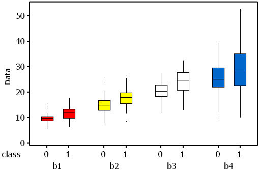
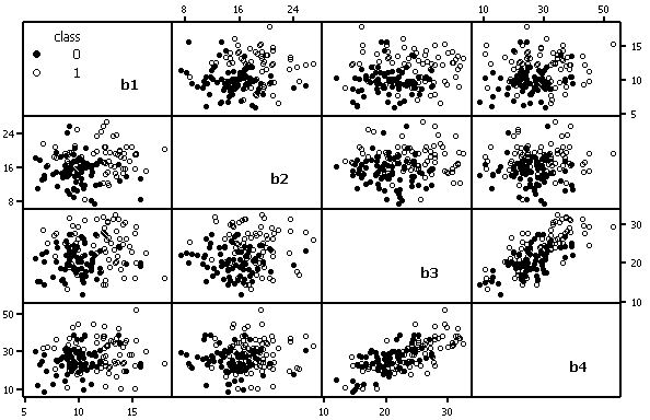 If effect sizes (difference in the means divided by the standard deviation) are
calculated it is possible to estimate the expected rank order for the standardised weights. In data set B
the expected order is (b1 = b3), b2 and b4 (see plot below for an indication of the amount of within-
variable variability, and the between-class differences).
If effect sizes (difference in the means divided by the standard deviation) are
calculated it is possible to estimate the expected rank order for the standardised weights. In data set B
the expected order is (b1 = b3), b2 and b4 (see plot below for an indication of the amount of within-
variable variability, and the between-class differences).
Analysis
This analysis was completed using SPSS V12.0. This is a direct entry analysis. In other words all of the predictors are included in the analysis.
The log-likelihood (LL) measures the variation in the class that is unexplained by the model. LLs are the logarithms of probabilities and, since probabilities are never greater than one, the logarithm will be negative. If the LL is multiplied by -2 (-2LL) the resulting measure, which is often called the deviance, approximates to a chi-square statistic and can be used to test hypotheses. At the start of the logistic modelling process the simplest model, the null model, has one term, the intercept or constant. The initial value for the intercept is loge(P(class=1)/P(class=2)). Large deviance values indicate a poor fit because there is a large amount of unexplained variation. As the model is developed, i.e. predictors are added, it is expected that deviance will decline. At the start of this model the deviance was 207.9, suggesting a very poor fit.
| Chi-square | df | Sig. | ||
|---|---|---|---|---|
| Step 1 | Step | 86.651 | 4 | .000 |
| Block | 86.651 | 4 | .000 | |
| Model | 86.651 | 4 | .000 |
The final model has a deviance of 121.3. This means that the change in the deviance has been 86.6 (207.9 - 121.3, see above). SPSS calls this the model chi-square and it is used to test a hypothesis that the predictors have improved the model by reducing the amount of unexplained variation. Since p << 0.05 there is strong evidence that the model, which includes the four predictors, has significantly reduced the unexplained variation.
The log-likelihood (-2 LL) can be converted into a pseudo-R2 statistics which measure the variability in the class that is explained by the predictors. Because the usual least squares R2 statistic cannot be calculated a range of pseudo-R2 statistics have been designed to provide similar information. SPSS reports two, the first being the Cox and Snell statistic, which tends to have a maximum less than one. Nagelkerke's R2 is derived from the previous one, but with a guarantee of a 0-1 range. Consequently it tends to have larger values. Values close to zero are associated with models that do not provide much information about class membership. In this analysis they are quite large (0.439 and 0.585) suggesting that over half of the variation in classes can be explained by the current predictors.
| Step | -2 Log likelihood | Cox & Snell R Square | Nagelkerke R Square |
|---|---|---|---|
| 1 | 121.293(a) | 0.439 | 0.585 |
| Step | Chi-square | df | Sig. |
|---|---|---|---|
| 1 | 2.459 | 8 | 0.964 |
If the significance value of the Hosmer-Lemeshow statistic is less than 0.05 it suggests that the model is a poor fit. In this analysis the p value of 0.964 indicates that the model adequately fits the data. The following table shows details of the fit between the observed and expected case frequencies in ten categories.
| class = 0 | class = 1 | Total | ||||
|---|---|---|---|---|---|---|
| Observed | Expected | Observed | Expected | |||
| Step 1 | 1 | 15 | 14.682 | 0 | .318 | 15 |
| 2 | 13 | 13.947 | 2 | 1.053 | 15 | |
| 3 | 12 | 12.570 | 3 | 2.430 | 15 | |
| 4 | 12 | 10.877 | 3 | 4.123 | 15 | |
| 5 | 9 | 8.846 | 6 | 6.154 | 15 | |
| 6 | 6 | 6.341 | 9 | 8.659 | 15 | |
| 7 | 4 | 4.353 | 11 | 10.647 | 15 | |
| 8 | 3 | 2.214 | 12 | 12.786 | 15 | |
| 9 | 1 | 0.944 | 14 | 14.056 | 15 | |
| 10 | 0 | 0.225 | 15 | 14.775 | 15 | |
The structure of a model is determined by the coefficients and their significance. The Wald statistic has an approximate chi-square distribution and is used to determine if the coefficients differ significantly from zero. The Wald statistic can be unreliable, with reduced values for the chi-square statistic. However, the significance of the coefficients can also be judged from the confidence limits for exp(b). A predictor that has no effect on the class has odds (exp(b)) of 1.0. Therefore, if the confidence limits include one (see b4 below) there is no evidence for a relationship between the predictor and the class. Confidence limits (95%) are calculated in the usual way, i.e. estimate ± z(0.05,2).se.
For example, for predictor b2 the lower confidence limit for Exp(b2) is e(0.355 - 1.96 x 0.08), which is e(0.1982) or 1.219. The upper confidence limit is e(0.355 + 1.96 x 0.08), which is e(0.5118) or 1.668. Because these limits do not include 1.0 there is evidence that the b2 contributes to the class of a case.
In this example it should be remembered that the lack of significance for b4 is related to its correlation with b3. Indeed, when used as a single predictor its coefficient is significantly different from zero and the confidence limits for exp(b) do not include 1.
| B | S.E. | Wald | df | Sig. | Exp(B) | 95% LCL | 95% LCL | ||
|---|---|---|---|---|---|---|---|---|---|
| Step 1(a) | b1 | 0.511 | 0.116 | 19.351 | 1 | 0.000 | 1.667 | 1.328 | 2.094 |
| b2 | 0.355 | 0.080 | 19.675 | 1 | 0.000 | 1.427 | 1.219 | 1.669 | |
| b3 | 0.349 | 0.084 | 17.191 | 1 | 0.000 | 1.418 | 1.202 | 1.672 | |
| b4 | -0.062 | 0.043 | 2.108 | 1 | 0.147 | 0.940 | 0.864 | 1.022 | |
| Constant | -17.487 | 2.856 | 37.483 | 1 | 0.000 | 0.000 | |||
| a Variable(s) entered on step 1: b1, b2, b3, b4. | |||||||||
The model can now be used to estimate, for each case, the probability that they belong to each class. For example, case 1 has values of 10.65, 16.92, 19.79 and 20.63 and is from class 0. These values can be substituted into the equation:
logit(case 1) = constant + b1x10.65 + b2x16.92 + b3x19.79 + b4x20.63
logit(case 1) = -17.487 + 0.511x10.65 + 0.355x16.92 + 0.349x19.79 - 0.062x20.63
logit(case 1) = -17.487 + 5.44 +6.01 +6.91 -1.28 = -0.407
p(class(case 1) = 1) = 1 / (1 + e-(-0.407)) = 0.400
p(class(case 1) = 0) = 1 - 0.400 = 0.600
If a 0.5 threshold, or cut-value, is applied this means that the predicted class for case 1 is class 0, the same as its actual class.
Once the predcited class membership has been estimated for each case the results can be presented in a table (confusion matrix) which cross-tabulates actual and predicted classes. In this example the number of misclassifications is the same for each class (14) and 81.3% of cases were correctly classified.
| Predicted class | Percentage Correct | ||||
|---|---|---|---|---|---|
| 0 | 1 | ||||
| Step 1 | Observed class | 0 | 61 | 14 | 81.3 |
| 1 | 14 | 61 | 81.3 | ||
| Overall Percentage | 81.3 | ||||
| a The cut value is .500 | |||||
Diagnostics
In all regression analyses it is important to check that there are no problems created by one or more of the cases that could invalidate the model. For example, if a case is substantially different from the rest in its class it may have a large effect on the model's structure and it should be investigated further. In the simplest situation the unusual values could be a consequence of incorrectly entered values.
Usually several diagnostic statistics, such as residuals and influence statistics, are calculated. Hosmer and Lemeshow (1989) suggest that all of them should be interpreted jointly to understand any potential problems with the model. The aim is to identify cases that are either outliers or have a large leverage. An outlier is an observation with a class value that is unusual, given the values for its predictor variables. This will result in it having a large residual. A residual is the difference between an actual and a predicted value. A case could also have an unusually small or large value for one of the predictors, which may cause it to have a large effect on the regression coefficients. The size of this effect is measured as the leverage of a case, a measure of how far its value for a predictor deviates from the predictor's mean. The combination of leverage and outlying values may produce cases that have a large influence. This will be apparent if they are removed because there will be large changes to the regression coefficients. However, it also important to recognise that a case with a large leverage need not have a large residual. Hence the need to consider both together.
There are many diagnostic statistics. For example, unstandardised residuals are simple differences between the observed and predicted classes, while standardized residuals (also known as Pearson or chi residuals) are the standardised residuals divided by an estimate of their standard deviation (actual value minus its predicted probability, divided by the binomial standard deviation of the predicted probability). Using the standard deviation as a devisor changes their probability distribution so that they have a standard deviation of one.
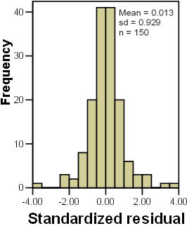
Standardized and studentized residuals should approximate to a normal distribution (N(0,1) and no more than 5% of the residuals should exceed |1.96| or approximately two. Similarly, <1% of the residuals should exceed |3.0|. The next plot shows that the standardised residuals have a good approximation to a normal distribution with a sufficiently small number of large residuals.
There are three main statistics that assess the influence that an individual case has on the model. The leverage (h) of a case varies from 0 (no influence) to 1 (completely determines the model).
Cook's Distance (D) also measures the influence of an observation by estimating how much the other residuals would change if the case was removed. Its value is a function of the case's leverage and of the magnitude of its standardized residual. Normally, D > 1.0 identifies cases that might be influential. Dfbeta, or dbeta, is Cook's distance, standardized and it measures the change in the logit coefficients when a case is removed. As with D, an arbitrary threshold criterion for cases with poor fit is dfbeta > 1.0. None of the cases in this analysis have a D value <1, suggesting that none of the case is creating problems.
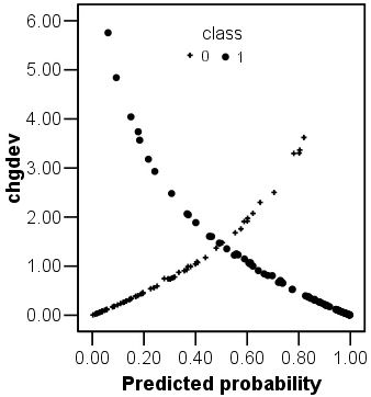
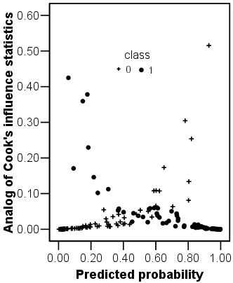
If the standardised residuals are squared the result is a change in the model's deviance arising from the inclusion of the case. Large changes in deviance indicate poorer fits. The plot opposite shows the change in deviance against the predicted class probability. There are two obvious curves on this plot, corresponding to the different classes. This plot could be used to identify the cases that are poorly fit by the model. In this example there are three or four class 1 cases that have large values for their change in deviance.
Accuracy
The earlier classification table suggested that the model had a class and overall accuracy of 81.3%. The calculator from the accuracy page estimates that Kappa is quite large (0.627).
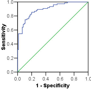
There are two main problems with these accuracy assessments. Firstly, they are based on the training data and are likely to be over-optimistic (see the accuracy page). Secondly, they assume that the 0.5 cut-point is appropriate. It is generally better to assess accuracy with a threshold-independent measure from a ROC plot. The ROC plot on the left has an AUC of 0.896 (std error = 0.025), with 95% confidence limits of 0.847 and 0.945. These figures suggest that the model is reasonably accurate.
There is a self assessment which re-analyses these data but with a portion of the data witheld for independent testing