This analysis uses the same data as that used in the first
logistic regression example. The results of the analysis (using SPSS 12.0) are
given below, followed by a series of self-assessment questions. For this analysis
the data have have been split, randomly, into 100 training cases and 50 test
cases. The training data have 47 class 0 cases and 53 calss 1 cases. In the test
data the frequencies are 28 and 22. You may wish to print this material before
attempting the questions.
Variables in the Equation
B
S.E.
Wald
df
Sig.
Exp(B)
Step 0
Constant
0.120
0.200
0.360
1
0.549
1.128
1
Omnibus Tests of Model Coefficients
Chi-square
df
Sig.
Step 1
Step
59.526
4
0.000
Block
59.526
4
0.000
Model
59.526
4
0.000
2
Analysis details
Decide which of the following statements are valid, with respect to this analysis.
Model Summary
Step
-2 Log likelihood
Cox & Snell R Square
Nagelkerke R Square
1
78.743
0.449
0.599
Hosmer and Lemeshow Test
Step
Chi-square
df
Sig.
1
3.482
8
0.901
Contingency Table for Hosmer and Lemeshow Test
class = 0
class = 1
Total
Observed
Expected
Observed
Expected
Step 1
1
10
9.788
0
0.212
10
2
8
9.093
2
0.907
10
3
8
8.000
2
2.000
10
4
8
7.047
2
2.953
10
5
6
5.401
4
4.599
10
6
3
3.802
7
6.198
10
7
3
2.172
7
7.828
10
8
1
1.193
9
8.807
10
9
0
0.432
10
9.568
10
10
0
0.072
10
9.928
10
3
Classification Table(c)
Observed
Predicted
Training Cases
Testing Cases
class
Percentage Correct
class
Percentage Correct
0
1
0
1
Step 1
class
0
38
9
80.9
19
9
67.9
1
8
45
84.9
3
19
86.4
Overall Percentage
83.0
76.0
a The cut value is .500.
4
Variables in the Equation
B
S.E.
Wald
df
Sig.
Exp(B)
Step 1(a)
b1
0.452
0.140
10.417
1
0.001
1.572
b2
0.463
0.123
14.222
1
0.000
1.589
b3
0.309
0.097
10.192
1
0.001
1.363
b4
-.072
0.053
1.896
1
0.169
0.930
Constant
-17.251
3.491
24.415
1
0.000
0.000
a Variable(s) entered on step 1: b1, b2, b3, b4.
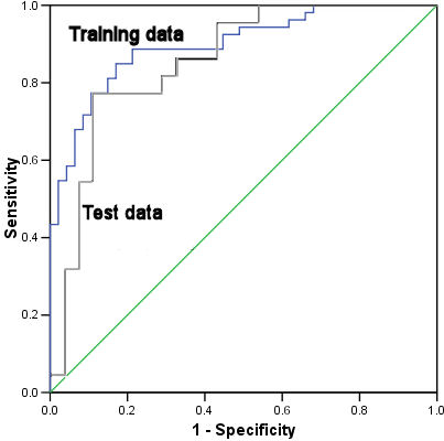
ROC Curve
5
AUC statistics
The AUC for the training data is significantly larger than the test data AUC.