Flow classification obtained from the visualizations
Relevant parameters to the classification:
r is the wave orbital amplitude a0 to ripple wavelength lr ratio
Ta is the Taylor number (refer to PhD for definition)
sr is the ripple slope defined as the ripple height hr over the ripple wavelength lr
σ is the wave angular frequency
T is the wave period
classification
Distinct types of flow patterns have been obtained. By filming from the side and from above the rippled section, two and three-dimensional patterns were visualized. The following pictures show the main types of flow pattern that were observed. At the bottom of this page a diagram shows the summary of the flow patterns obtained.
Note: for all the side view sequences, the waves always propagate from the left to the right.
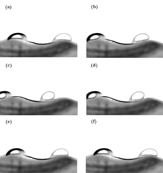
Roll pattern
For weak flow conditions (r < 0.5) and usually for a gentle ripple slope, this type of pattern was observed. The rolls gently oscillate around each crest.
(side view)
sr = 0.1; r = 0.18; T=
1.43 s; (a) σt = 0; (b) σt = 2π / 5; (c) σt = 4π / 5;
(d) σt = 6π / 5; (e) σt = 8π / 5; (f) σt = 2π; all wave phases are relative
phases.
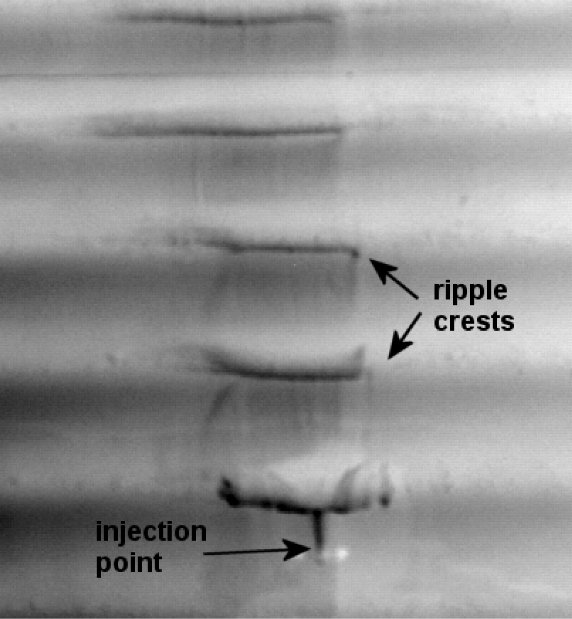
This pattern is typically two-dimensional as no particular structure was seen from above (as shown in the picture below).
(top view)
Roll plus jets pattern
For a stronger r than for the roll regime, and / or usually for steeper ripple slopes, jets of dye tend to appear on the lee-side of the ripple crests. The rolls of dye are still present, and oscillate around each crest.
(side view)
sr=0.175; r = 0.17; T = 2
s; (a) σt
= 0; (b) 2π
/ 5; (c) 4π
/ 5;
(d) 6π
/ 5; (e) 8π
/ 5; (f) 2π
; (g) 12π
/ 5; (h) 14π
/ 5; (i) 16π
/ 5; (j) 18π
/ 5.
This pattern is typically two-dimensional as no particular structure was seen from above (as shown in the picture below).
(top view)
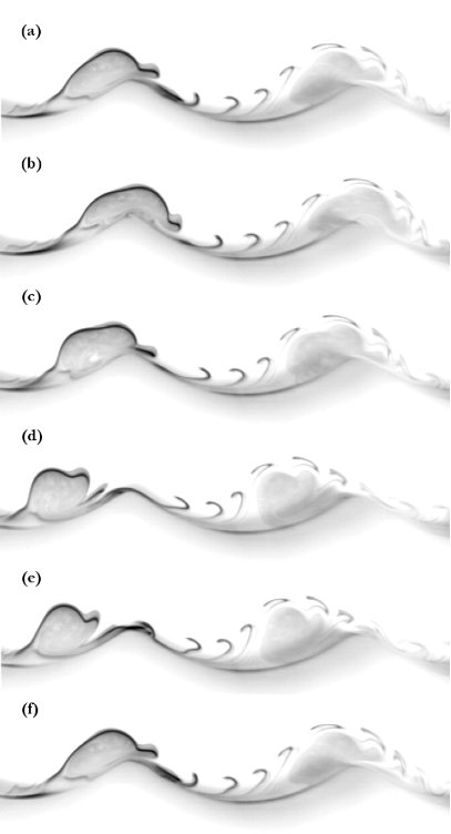
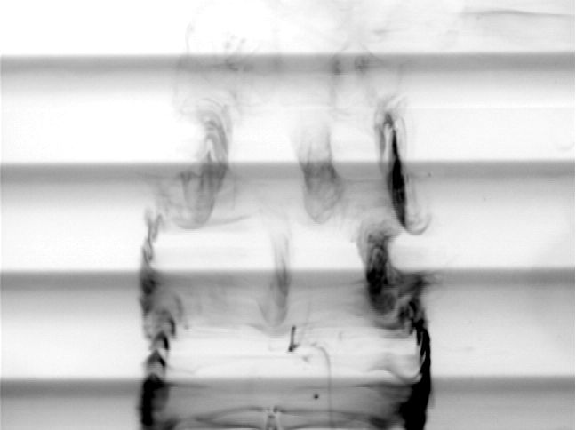
Vortex ejection pattern
A vortex is created and ejected at each half wave cycle.
(side view)
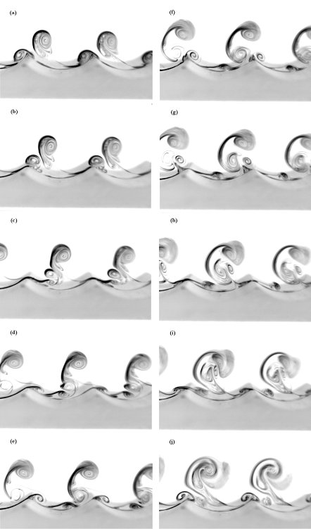
sr = 0.175; r = 0.46; T = 2.5
s; (a) σt = 0; (b) π / 5; (c) 2π / 5; (d) 3π / 5; (e) 4π /5; (f) π;
(g) 6π / 5; (h) 7π / 5; (i) 8π / 5; (j) 9π / 5.
----------------------------------------------------------------------------------------------
click here to view a video showing the vortex ejection process
for the case: s = 0.175; r = 0.35; T = 2 s
----------------------------------------------------------------------------------------------
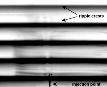
This regime was three-dimensional for around 90% of the cases visualized.
Among these 3D cases, about 70% of them showed from above a type of structure called "rings", as shown below:
(top view)
By measuring the instability wavelength of these rings, the following curve can plotted:
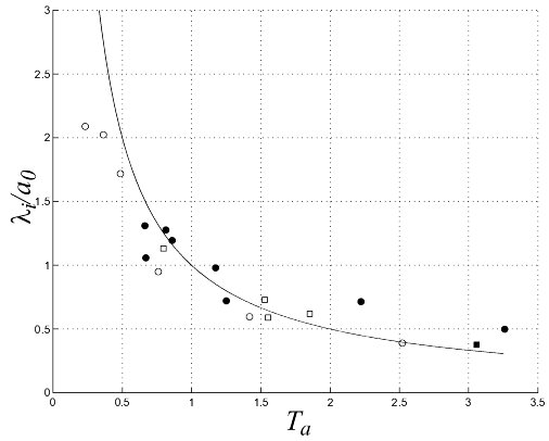
Ratio of ring instability wavelength λi to wave orbital amplitude a0 for the ring pattern.
Experimental data: ○ sr = 0.175; ● sr = 0.12; □ sr = 0.1; ■ sr = 0.05. The curve is λi / a0 = 1 / Ta.
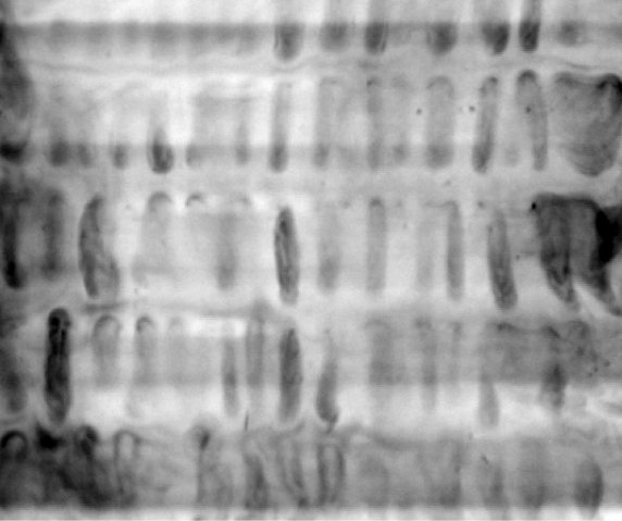
Brick-pattern
For about 15% of the 3D cases obtained, a pattern called Brick pattern was obtained. The transverse bridges are different from the one observed in the ring regime as they are shifted of approximately half their wavelength from one crest to another. A schematic representation of brick-pattern ripples that could be expected when such instabilities take place is shown below. The black areas represent the transverse bridges, shifted from one crest to another.
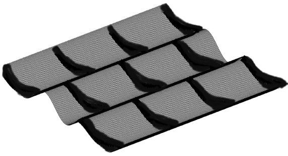
Schematic representation of brick-pattern ripples.
(top view)
Brick pattern flow structure; sr = 0.175; T = 2 s; r = 0.23.
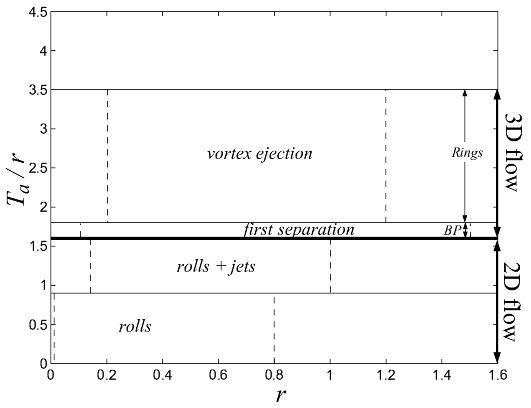
Flow characteristics summary
The thicker line shows the separation between 2D and 3D flows. BP: area where 3D brick patterns were observed. Rings: area where 3D ring structures were observed. The area noted first separation corresponds to the cases where the flow separates but the vortex ejection was not clearly visualized. The area above the upper limit of the vortex ejection area could not be studied due to the presence of turbulence limiting the experimental visualizations. The dashed lines show the range in r for which each regime was obtained. Areas outside the dashed lines domain could not be studied due to the appearance of turbulence limiting the visualizations. The horizontal thin lines are for visual help and are arbitrary.