Chapter Two
Problem Background
2.1 The Weber Problem, in general
The Weber Problem is a simple location science problem in facility location, defined in a two dimensional space with Euclidean (L2) geometry. It is also known as the planar Euclidean minisum distance single facility location problem, which adequately defines its characteristics. It is also known as the spatial median problem, as it attempts to locate the median location of a new facility with regards to existing weighted demand locations. For the Weber problem, each existing (hereafter demand) point is assigned an arbitrary non-negative weight, which can be considered a measure of the demand's relative importance or 'travel' cost.
The Weber problem is optimally solved using an algorithm designed by Weiszfeld (34 or 35). Weiszfeld's algorithm is a gradient steepest descent iterative method, shown first in a 1936 paper in French (no attempt is made to translate). (There exists some contention as to which Weiszfeld reference is correct, and both the 1936 and 1937 papers are included in the bibliography.) The objective function for the L2 planar minisum problem,
min f(x,y)=∑wi[(x-ai)**2+(y-bi)**2]**1/2 [2]
is strictly convex unless the demand points are collinear, in which it is only convex. If the function globally minimizes at a demand point (a majority theorem case or an irregular point), there is no need to apply Weiszfeld; otherwise, the procedure partially differentiates the distance metric equations and solves them for equality to zero. For the L2 Euclidean metric in integer n-space the result is a global minimizing point.
2.2 Problems in Spherical Geometry: Non-Convex Objective Functions
Hull convexity is a simple and basic concept to location science. The convex hull of a location problem is a space containing all demand points, with extreme points (corners, in L2 space) defined by demand points. The shortest path between any two points must lie fully inside the convex hull, or the distance metric is not convex for that space. A simple planar example shows this well:
Figure 1. Convex and Non-Convex Hulls on a Plane
In the first diagram, the shortest L2 distance between any two points A and B lies completely within (or along the edges of) the rectangular hull. If instead we define a space in the second diagram and place points A and B in the closed corners, we see that the shortest L2 distance between the points leaves the space. This is not a convex hull for L2 distances.
A mathematical definition is presented in Litwhiler (25): "A set C in S**2 is said to be convex if for each two points x and y in C such that 0<p(x,y)<Π then the segment xy [is contained in set] C. The convex hull of a set A in S**2 is the intersection of all convex sets containing A" (p142). For spherical geometries, the continuation of this discussion leads to the conclusions drawn from inspection of Figures 2 and 3: "The convex hull of 2 points is either a segment or the two points themselves; the convex hull of a closed hemisphere and a point not on it is the entire sphere S**2" (p142). The confusion when dealing with great circle arc distances is due to the non-differentiability of the combined trigonometric function describing arc distance ai(Φ,Θ). Although the convex hull of a greater-than-hemispherical set of points is the entire sphere, the objective function is not convex over the convex hull, leading to the difficulties discussed below.
The Weber problem on a sphere utilizing great circle arc distances as the distance metric is not convex. This can be shown by considering the concept of hull convexity and a visualization of the sphere; for a spherical circle with center at a pole (for convenience), the spherical circle consists of all points within a given arc distance from that center (lines of latitude defining the circle's possible edges). For convexity to apply to a space for a given norm, the shortest norm distance between two points in the space must be completely contained within the space. It is obvious that if a spherical circle is of radius greater than Π/2 (one hemisphere), for two points just on that circle's radius the shortest arc distance will leave the spherical circle and thus the convex space. Therefore, the largest convex space on the surface of a sphere must be a hemisphere.
It is not enough for a problem to be in a spherically convex space to assure global optimality, however. Drezner and Wesolowsky (16) prove, via an error inducing experiment, that the maximum spherical circle radius insuring a minimum point's global optimality is of radius Π/4. Litwhiler (25) also states this as a conjecture in his seminal paper, based on the following assumptions: There exists (one or more) globally optimal solution(s) within the convex hull, and that the objective function for a certain region is unimodal. So long as the demand points are not "collinear" (located on the same great circle), the proof is shown by defining the maximum region over which the combinatorial trigonometric distance metric is strictly unimodal. Covering circles larger than this may have (but not necessarily) alternative local optima that can trap optimization algorithms at sub-optimal solutions. Covering circles meeting the criteria (all demand points within an inclusive spherical covering circle of radius p/4) will have a single, unique, and global minimum point. No analysis of the multimodality of the distance metric for larger spherical covering circles is attempted in this research.
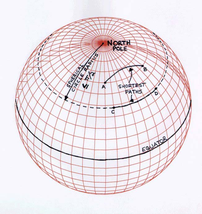
Figure 2. Non-Limiting Conditions to Convexity on a Sphere
In Figure 2, a spherical-surface set of demand points is transformed such that the center of the covering circle is centered at the North Pole. The covering circle is of radius equal to or less than Π/2 radians (less than or equal to one hemisphere). All shortest paths (minor great circle arcs) connecting any set members are either within (points A and B) or on the edge of (points C and D) the covering circle, and therefore the problem is determined to be convex. Note that the increase of the a covering circle's radius from Π/4 to Π/2 radians from the previous discussion on a single, unique minimizing point has no bearing on that discussion. There will still be a globally minimum point (or points) if the circle's radius is so increased, but there may also be local minimum points. The existence of these local points in no way affects the convexity of the problem.

Figure 3. Hemispherical Limit to Convexity on a Sphere
In Figure 3, another spherical-surface set of demand points is also transformed to be centered at the North Pole, but the covering circle radius for the set is strictly greater than Π/2 radians (a larger area than the northern hemisphere). Many possible shorter paths may still lie wholly within the covering circle. Points A and B, each just inside the covering circle's edge, may have a shortest path that extends outside the covering circle's boundary, and points C and D, on the edge of the covering circle, have a shortest path that is entirely outside the covering circle (except for the endpoints, of course)! These paths are clearly outside the area that could otherwise be described as convex, so the problem is determined to be non-convex.
2.3 Norms for Use in Spherical Weber Problems
Normal L2 Euclidean distances, D=[(x-ai)**2+(y-bi)**2+�]**1/2, are true shortest path distances in the normal n-spaces we typically operate in. The shortest path between two points, say your couch and your refrigerator, is a straight line. However, because there may be a wall, stairs, or furniture between you and your beer, you may have to use another metric to get there. Graph and network space applications of these norms are not considered in this research. Similarly, because the true shortest path between New York and London would cut under the Atlantic Ocean and through the crust and mantle of the earth, it is not currently feasible to take this path.
The standard metric for distance determination on the surface of a sphere is the great circle or shortest arc distance is
D= Α * arccos(cos(Φ1)*cos(Φ2)*cos (Θ1-Θ2)+sin(Φ1)*sin(Φ2)). [3]
When vertical distance changes over the spherical surface are neglected, it provides a true shortest path distance. It is the best metric for measuring true distances over large (>1 degree of arc) distances on the earth. However, because of the trigonometric functions involved, it is multi-modal for regions encompassing more than Π/4 radians of spherical radius.
The centroid problem, a variation on the Weber problem, uses squared-Euclidean distances as the distance metric. The 3-D objective function for this problem is
F(x,y,z)=∑wi[(x-ai)**2+(y-bi)**2+(z-ci)**2]. [4]
Litwhiler (25) attempted to develop two algorithms for the Weber problem on the sphere. Recognizing that he needed to obtain a starting solution to work from, he tried several approaches, including random starts, demand point starts, and projected centroid starts. The projected centroid starting solutions in his test cases tended to provide 'good' points and were often in the vicinity of the global minima; the original work leading to the projected centroid was done by Wendell in 1971 (36). Utilizing an approximation of the objective function based upon
arcsin(y) =(approx) Πy**/2, y [within] [0,1] (a substitution of Πsin2(ai(Φ,Θ)/2) for arc distance ai(Φ,Θ)), [5]
Wendell formulated the normalized approximate solution (in R3) to the problem as
x0*(x,y,z)=(∑wiP(Xi))/((∑wiP(Xi))**2+(∑wiP(Yi))**2+(∑wiP(Zi))**2)**0.5,
(∑wiP(Yi))/((∑wiP(Xi))**2+(∑wiP(Yi))**2+(∑wiP(Zi))**2)**0.5,
(∑wiP(Zi))/((∑wiP(Xi))**2+(∑wiP(Yi))**2+(∑wiP(Zi))**2)**0.5. [6]
Litwhiler (25) shows that this approximate solution is actually the projected centroid, and can be sometimes useful as a starting point.
2.4 Existing Methodologies for Global Minimization
The seminal paper for this area of research should be considered to be Litwhiler's doctoral dissertation (25). Several other researchers had worked in the field, but with unconnected results. Litwhiler worked on both minisum and minimax problems, for both single- and multi-facility location problems. His work spawned the large number of papers attempting to tie down the ends throughout the 1980s (the majority of the resources used per this research's bibliography).
As discussed in section 2.3, Litwhiler used the projected centroid as a starting solution for his algorithms. He discussed also using the projected R3 1-median, but discounted it because of the costs of computing it due to the iterative nature of the problem. Random start points and demand/antipodal start points were also discussed; the limited computing power available to him was apparently one reason the benefits of using each start point technique were not discussed in any greater detail.
The projected R3 1-median as a starting point has therefore been discussed in the literature, but not apparently pursued; since we now have the processing power to make simple iterative calculations like finding the 1-median to a reasonable degree of accuracy rapidly, it may be of interest to determine how that projection relates to both the global minima and projected centroid in a number of cases. This thesis provides this analysis.
Next Page
Back to Index