Introduction
The Problem
As described in the paper, this project tries to solve the problem of human detection, even in cluttered backgrounds under difficult illumination.The ability to detect and tell whether and where a human exists in an image, could be helpful for many kind of entities (Image search engines, security companies and more...).
This project is an implementation of the algorithm described in the paper, including another application which evaluates the solution in the wild.
Related Paper
Our work related to HOG feature extraction is fully based on the paper:Histograms of Oriented Gradients for Human Detection, Navneet Dalal and Bill Triggs, CVPR 2005
Our Work
Our aim in this work, was:- To implement our own HOG feature extractor (according to the algorithm description in the paper)
- To train a classifier on the dataset which was prepared and used by the authors of the paper, and to get high accuracy on the corresponding testing set
- To create a program which evaluates the classifier in the wild, in a way that it scans images provided by the user and uses our trained classifier to detect humans within those provided images
Used Datasets and Technologies
The Used Dataset
We used the INRIA Person Dataset, which was prepared by the authors of the original paper we base onAbout the dataset:
- A 970MB tar archive file, named INRIAPerson.tar
- Contains the following relevant directories:
| 96x160H96/Train/pos: | 2416 human images centered and cropped, used as positive training set (each image is sized 96x160 pixels) |
| 70x134H96/Test/pos: | 1132 human images centered and cropped, used as positive testing set (each image is sized 70x134 pixels) |
| Train/neg: | 1218 images with no humans within. Image sizes vary. We used them to randomly crop and save 24360 patches (20 patches from each), to be used as a negative training set |
| Test/neg: | 453 images with no humans within. Image sizes vary. We used them to randomly crop and save 9060 patches (20 patches from each), to be used as a negative testing set |
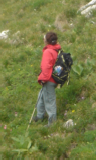
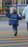
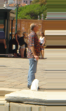
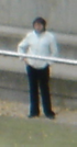
Some samples from the dataset:
| 96x160H96/Train/pos: |


|
| 70x134H96/Test/pos: |


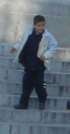


|
| Train/neg: |
|
| Test/neg: |
|
The Used HOG Feature Vector Extractor
The HOG feature vector extractor is implemented in Matlab, in the function computeHOG126x63(). Its implementation is found in the file computeHOG126x63.m- The function computeHOG126x63() expects an image sized at least 63x126 pixels
- It assumes that a human is centered in the provided image (if it is a positive sample) and it computes the HOG feature vector only on the sub-image formed by the central 63x126 pixels
- The usage of 63x126 pixels for a human image, is because according to the paper, a cell size should be 6x6 pixels and a block size should be 3x3 cells.
It means that a block size is 18x18 pixels. As according to the paper, blocks should have 50% overlapping, we need width and length that are divisible by 9.
Hence, we chose 63x126 pixels, in which both width and height are divisible by 9 and which are the closest such dimension to 64x128 pixels, suggested in the paper
The Used Classifier and Related Libraries
- The training and classification code is written in C
- We used a FeedForward neural network as a classifier, from the library: C/C++ Neural Network
- As the feature vectors are computed and exported by Matlab into CSV files, we also had to use a CSV parser library: C/C++ CSV Parser
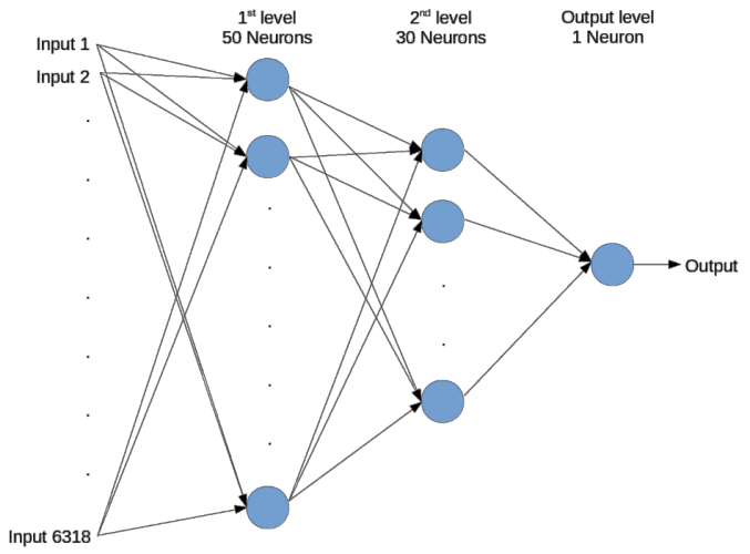
- Our FeedForward neural network is set with the following structure and behavior:
- 6318 inputs (The length of the feature vector)
- 50 neurons as a 1st hidden level
- 30 neurons as a 2nd hidden level
- 1 output neuron
- All the neurons are activated with TANH function
The Workflow
The following diagram explains our workflow in a very high level: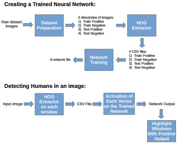
Note: CSV stands for "Comma Separated Values"
For example, the below sample content of a CSV file defines the 3 vectors [1 2 3] , [1.23 0.54 -6], [-1 -1 -1]
1,2,3
1.23,0.54,-6
-1,-1,-1
1.23,0.54,-6
-1,-1,-1
Thus, we can compute the HOG vectors of many images and then export them all at once into a CSV file.
This CSV file can be parsed an be used by other applications, such as our C application for training and activating neural networks
Dataset Preparation
As explained in the Used Dataset part, not all of the dataset images are ready to use:The most simple case, is with the positive samples (both for training and for testing):
- A human is centered in each of the positive sample images (Explained in the Used Dataset part)
- As explained in the Used HOG Feature Vector Extractor part, our function for HOG feature vector extraction always takes only the sub-image formed by the central 63x126 pixels
- It actually means that in our case, the positive samples do not require any preprocessing, as our function will anyway process only the relevant part of each of these samples
The more challenging case, is the preparation of the negative samples:
- We want the negative training set to be ~10 times larger than the positive one
- As the positive training set contains 2416 samples, while there are 1218 large negative training images with no human within, we randomly crop 20 patches of 63x126 pixels each, from each of the 1218 large negative images
- This cropping gives us a negative training set, which contains 24360 samples sized 63x126 each
- The same is done with the negative testing set: there are 1132 positive testing samples and 453 large negative testing images.
We again randomly crop 20 patches of 63x126 pixels from each large negative image, to form a negative testing set of 9060 samples
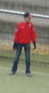
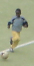
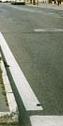
Here are some samples of the negative patches we randomly cropped from the large images:
| Training negative samples: |


|
| Testing negative samples: |


|
Finally, the dataset we are going to use is formed by:
| 2416 positive training samples: | Taken without preprocessing from 90x160H96/Train/pos |
| 24360 negative training set | Prepared by cropping patches from 1218 images from Train/neg |
| 1132 positive testing samples | Taken without preprocessing from 70x134H96/Test/pos |
| 9060 negative testing samples | Prepared by cropping patches from 453 images from Test/neg |
We copy these photos we prepared into 4 directories, so we can easily access them later:
- train/pos - 2416 positive training images
- train/neg - 24360 negative training images
- test/pos - 1132 positive testing images
- test/neg - 9060 negative testing images
Note: The cropping of the negative images into samples is performed by our implemented Matlab function cutRandomImages(). To automatically cut and save 20 patches per image from source images directory SRC into destination images directory DST, where each patch is sized 63x126 pixels, one should call it as cutRandomImages(SRC, DST, 20, 63, 126)
This function is found in the file cutRandomImages.m
Extracting HOG Feature Vectors from the Dataset
After the Data Preparation step, we have 4 directories of images, which we want to turn into HOG vectors.We use our Matlab function createDataset() in order to turn the images into HOG vectors and to save them in corresponding 4 CSV files.
Our function createDataset() gets 2 parameters:
- Input images directory
- Output CSV file
For example, to create a CSV file of the positive training samples, we'll call the function with the path to the train/pos directory and with a path to an output file, which we'll name something like train_pos.csv.
In general, the flow of the function createDataset() is:
- Get all the images that are in the provided input image directory
- prepare a matrix sized Nx6318 (where N is the number of found input images)
- For each image, call the function computeHOG126x63() so it computes a 6318 sized HOG vector of that image, and save this vector as a line at the matrix
- Finally, when the matrix rows contain all the HOG vectors, output the matrix into the provided output file, in CSV format
Below is a detailed explanation of the HOG extraction flow.
Given a 63x126 pixels image, our HOG feature extractor works according to the following flow:
- If the provided image is not in Grayscale, convert it to Grayscale
- Compute the image X-gradient matrix using convolution with the mask: [-1 0 1]
- Compute the image Y-gradient matrix using convolution with the mask: [-1 0 1]' (the ' operator stands for transpose)
- For each pixel in the image, compute its gradient magnitudes matrix, using the computed X and Y gradient matrices. The gradient magnitude in pixel (i,j) is defined by the formula:
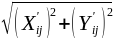 , where X' and Y' stand for our computed X-gradient matrix and Y-gradient matrix respectively
 - For each pixel (i,j) in the image, compute its gradient directions matrix, using the formula:
 , where again, X' and Y' stand for our computed X-gradient matrix and Y-gradient matrix respectively
 - As the arctan() function returns values between -90° and 90°, while we want the directions to be between 0° and 180°, we add (+180°) to all the negative values (we actually "flip" the negative angles to the other side). More information about it is in the notes below
- Iterate over all blocks sized 18x18 pixels, with 50% overlapping between each block, and do:
- Divide the block into a grid of 3x3 equal cells (such that each cell is formed by 6x6 pixels)
- Iterate over the cells, and do:
- Allocate a new array with 9 indices
- Compute the sum of all the gradient magnitudes of all the pixels with gradient direction between 0° and 20°. Assign this value to the 1st index in the allocated array
- Compute the sum of all the gradient magnitudes of all the pixels with gradient direction between 20° and 40°. Assign this value to the 2nd index in the allocated array
- . . .
- Compute the sum of all the gradient magnitudes of all the pixels with gradient direction between 160° and 180°. Assign this value to the 9th index in the allocated array
- ## Note: This cell processing is actually a computation of a 9-binned Histogram of Oriented Gradients for this specific cell. We divided the range of 0° to 180° into 9 equal bins of 20° each, and summed the magnitudes for each bin from the pixels of the 6x6 pixels sized cell
- Concatenate all the cells' arrays into one array with 81 indices (one cell's array has 9 indices and there are 3x3 = 9 cells ==> there should be 81 indices in the concatenation of the arrays)
- ## Note: the new array we just formed by a concatenation of the arrays of all the cells in the block, is actually the Histogram of Oriented Gradients of this block
- Normalize the 81-sized array by dividing it by:
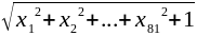 , where x is the array. This normalization is done in order to remove the effect of local lights differences
 - Concatenate all the blocks' 81-sized vectors into 1 long vector with 6318 indices (There are totally 78 blocks of 18x18 pixels each and with 50% overlapping, while each block's vector has 81 indices, hence, the final vector has 78 * 81 = 6318 indices)
- Output the vector sized 6318 as the HOG feature vector of the provided image
The following graphical slideshow might help to understand it better:
Notes:
- In the paper, it is reported that the best results were received when the gradient directions where unsigned (i.e. between 0° and 180°)
- When calling the function arctan(x/y), it first computes the value of x/y and then it calls arctan() with this computed value. It means that arctan() loses information, as e.g. if its argument is positive, it can't know whether it was (+/+) ==> [0°,90°] or (-/-) ==> [180°,270°]. The same happens when the argument is negative - it can't know whether it was (-/+) ==> [90°,180°] or (+/-) ==> [270°,360°]. Hence, in Matlab, it returns values only between -90° and 90°. It means that we anyway get the results as we want them to be, except for the fact that for negative values, we get the results between -90° and 0°, instead of between 90° and 180°. Hence, we "flip" all these negative angles by adding (+180°) to each of them. It finally lets all our results be in the range of 0° to 180°
Training and Evaluating the Classifier
The training and classification processes are done in a C application.The training process:
After the Extracting HOG Feature Vectors from the Dataset step, we have 4 CSV files:
- train_pos.csv - contains 2416 CSV lines
- train_neg.csv - contains 24360 CSV lines
- test_pos.csv - contains 1132 CSV lines
- test_neg.csv - contains 9060 CSV lines
We are going to train the network, in a way that we'll want each activation of a positive sample on the network to output 1.0, and each activation of a negative sample on the network to output (-1.0).
As the negative training set is more than 10 times larger than the positive training set, we will each time train the network on a positive sample, and then on 10 negative samples, until we finish with all the positive samples.
It means that we actually give up the last 200 negative training samples, as we are going to use only 24160 of them (which is 10 time the size of the positive training set).
It also means that finally each training epoch will consist of 2416 + 24160 = 26576 training iterations.
In order to accelerate the training, we use the FeedForwardNetwork API function FeedForwardNetwork_train_fast() instead of the standard function FeedForwardNetwork_train().
The function FeedForwardNetwork_train_fast() accelerates the training in a way that it lets the user define a callback function, which tells whether the output is satisfying. If the answer is positive, it skips the backpropagation and weight updating over the network, and thus it saves a lot of computation time.
We define this callback function to return positive answer if the sample is positive and the network output is greater than 0.5, or if the sample is negative ant the network output is less than 0.5. Other cases yield negative answer, which will cause the API to update the weights of the network using Backpropagation algorithm.
The flow of the training process is the following:
- Read each of the CSV files into an array of arrays of doubles (See external link to C/C++ CSV Parser)
- Create an instance of a FeedForward neural network, as described in The Used Classifier and Related Libraries, with learning rate of 0.01
- "forever" do:
- Iterate over the positive training samples (there are 2416 such), and do:
- Call the training function on the current positive sample
- Call the training function on the 10 corresponding negative samples
- Check the network performances over the testing set, and if it is the best performances until now, save the network into a file (Using the API function FeedForwardNetwork_saveToFile())
- Kill the process when the network is fully trained on the training set, such that the results stop changing
The evaluating process:
This step is much simpler than the training process, as now we already have a trained network.
We get from the user a path to a CSV input file and a path to a trained network file.
The flow of the evaluating process is the following:
- Read all the input HOG vectors from the provided CSV file into an array of arrays of doubles (again using C/C++ CSV Parser)
- Create an instance of a FeedForward neural network using the trained network file (Using the API function FeedForwardNetwork_new_from_file())
- Iterate over the HOG vectors, and do:
- Activate the vector on the network using the API function FeedForwardNetwork_activate().
- If the output is greater than 0.5, print "1", else, print "0"
Each output line contains one of the numbers {0, 1}, such that 1 is a positive answer and 0 is a negative answer, where of course, the result in the i'th output line is corresponding to the sample represented by the HOG vector at the i'th line in the provided CSV file
Using the Classifier in the Wild
After training and testing the classifier using the dataset, we also wanted to check how effective it is when its desired to detect humans within some random image.Note that the negative training and testing set we used, contain patches from a lot of human-free various images.
We assume that the amount of non-human-objects, which their HOG looks similar to a human's one, is pretty small in these random images.
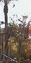
Though, some objects with strong vertical components like trees, poles and human limbs could produce HOG descriptors that are very similar to humans' ones and that are too hard to discriminate from real humans.
The following work we've found supports this claim: Pedestrian Detection project (Computer Vision course, Computer Science Department in Stanford University)
Basing on this assumption, we do not expect to see the same accuracy on each random image that is going to be checked. Some images could give better results, while others could give worse, depending on the contents of the image.
Of course, we expect the accuracy rates to tend to the results we reported on the testing set, when measuring and summarizing them on a large enough amount of scanned random images.
Our detector works in the following way:
- It computes the HOG vector all the 63x126 windows with 80% overlapping in the input image
- Then, checking all windows with size multiplied by sqrt(2). We downscale them to our 63x126 size and compute also their HOG vectors
- We continue the same way with window sizes always multiplied by sqrt(2), until we reach the limit of the height or the width of the image
- We then output all the window's HOG vectors into a CSV file and then we call the classifier
- The classifier activates each input vector on the network, and returns a positive result if the output of the network was greater than 0.5, and a negative result otherwise.
- The corresponding windows of all vectors which got a positive result from the classifier are highlighted with green border
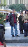
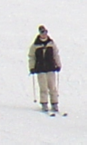
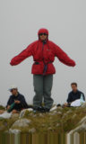
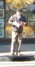
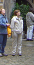
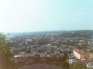
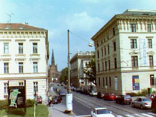
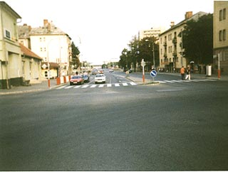
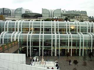
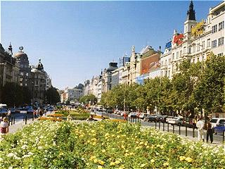
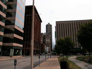
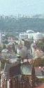
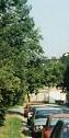
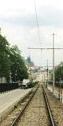
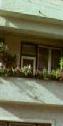
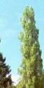
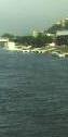
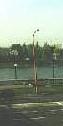
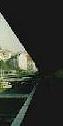
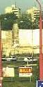
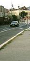
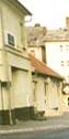
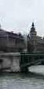
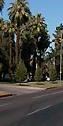
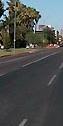
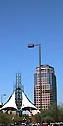
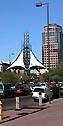
Here are some results we got:
| A perfect performance. 100% accuracy |
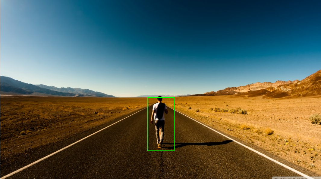
|
| An excellent performance. Only 6 false-alarms out of thousands of checked windows. Less than 1% of mistake |
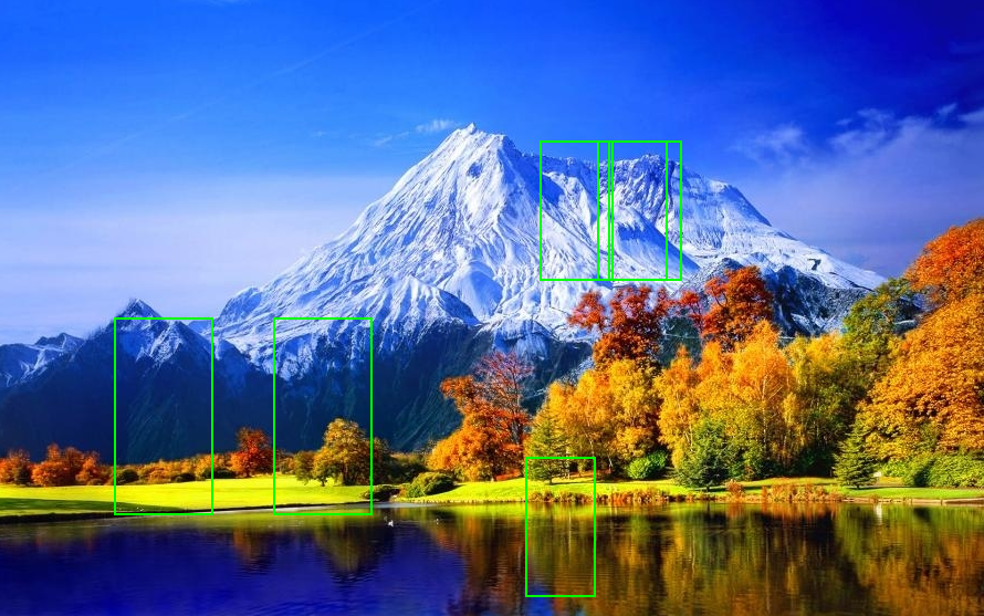
|
| In a crowded street, the results are more noisy and harder to read. However, all the humans (sized at least 63x126) were detected and the rate of false-alarms is less than 2% of the thousands of checked windows |
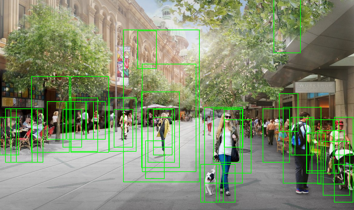
|
| In another less crowded street, most pedestrians were detected, and again we can spot a few false-alarms |
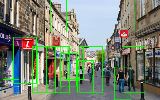
|
Results
As mentioned in the dataset preparation section, we had 1132 positive samples and 9060 negative samples in the testing set.We start with showing a ROC curve that describes the results:
A high-scope ROC curve graph
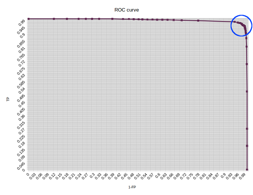
A zoom on the ROC curve interesting area (The area in the blue circle above)
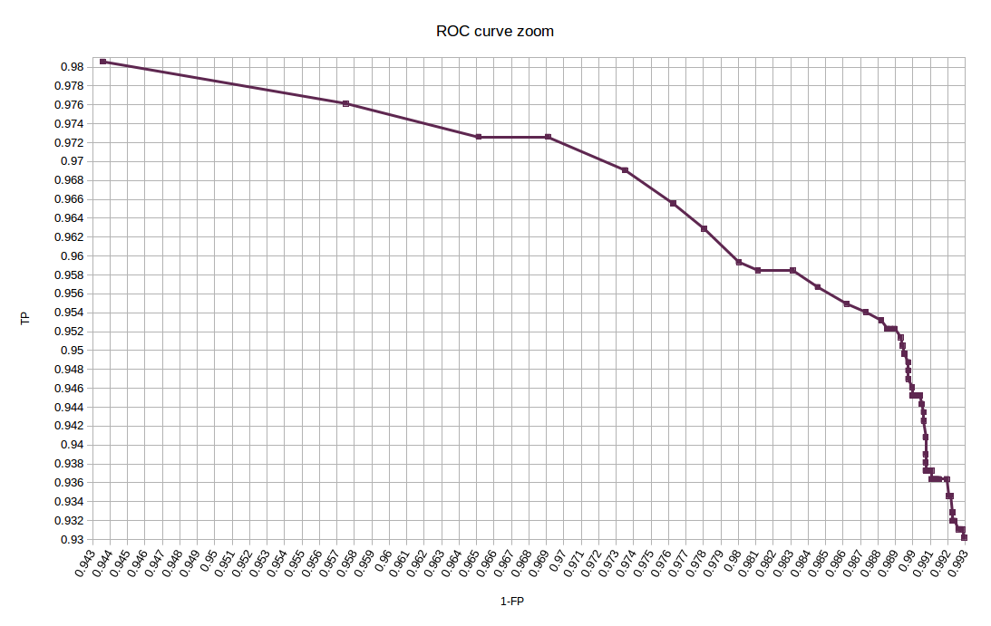
Below is also a confusion matrix, calculated with threshold 0.66, which is the one that yields the highest accuracy with the testing set.
The performances we got are given in the following confusion matrix:
| Predicted Class | |||
| Human | Non-Human | ||
| Actual Class |
Human | TP 1054 (93.11%) |
FN 78 (6.89%) |
| Non-Human | FP 65 (0.72%) |
TN 8995 (99.28%) |
|
Using these values, we can compute precision, recall and other scores:
| Precision: | 99.23% | [TP / (TP + FP)] = [0.9311 / (0.9311 + 0.0072)] |
| Recall: | 93.11% | [TP / TP + FN] = [0.9311 / (0.9311 + 0.0689)] |
| Accuracy: | 98.6% | [(TP + TN) / (P + N)] = [(1054 + 8995) / (1132 + 9060)] |
| F1 Score: | 96.07% | [2TP / (2TP + FP + FN)] = [(2 * 0.9311) / (2 * 0.9311 + 0.0072 + 0.0689)] |
| Magnitude: | 96.22% | [sqrt(precision^2 + recall^2)] / sqrt(2)] = [sqrt(0.9923^2 + 0.9311^2) / sqrt(2)]
Note: the magnitude is divided by sqrt(2) to get a result between 0 and 1 |
Related Files
All the files we wrote and used, including our trained network, are available here.Note that we could not include here the processed negative dataset, as its size is too big.
Note that the C code was tested only with GCC compiler in Unix. Though, with small changes, it should work also on MSVC.
Relevant files:
-
createDataset.m
Used for creating a CSV file of HOG vectors out of a directory if images -
cutRandomImages.m
Used for randomly cutting and saving patches from a directory of large images into a target directory -
computeHOG126x63.m
Used for computing a HOG vector of the subimage formed by the central 63x126 pixels of the provided image -
detectHumans.m
Used for scanning windows in a large input image and evaluating the classifier on them, in order to highlight detected humans -
train.c
Used for creating, training and saving a FeedForward neural network that is trained on the dataset -
evaluate.c
Used for evaluating vectors on a trained network and returning True/False
External Links and Resources
- The paper: Histograms of Oriented Gradients for Human Detection, Navneet Dalal and Bill Triggs, CVPR 2005
- The dataset: INRIA Person Dataset
- A C library for parsing CSV files: C/C++ CSV Parser
- A C library for working with neural networks: C/C++ Neural Networks
Credits
This project was prepared by Tal Hakim and David Cohn, students for M.Sc. degree in Computer Science in University of Haifa, Israel, as an assignment in the course Recognition and Classification in Images and Videos, taught by Dr. Margarita Osadchy, 2015.The project is based on the paper: Histograms of Oriented Gradients for Human Detection, Navneet Dalal and Bill Triggs, CVPR 2005