Height Spreadsheet

Lesson1

Purpose: students will be able to use the F2 shortcut to place insertion point, add data, make data bold, merge and center data, do the Sum, Average, Max, Min, and Count formula.

1. Excel>open
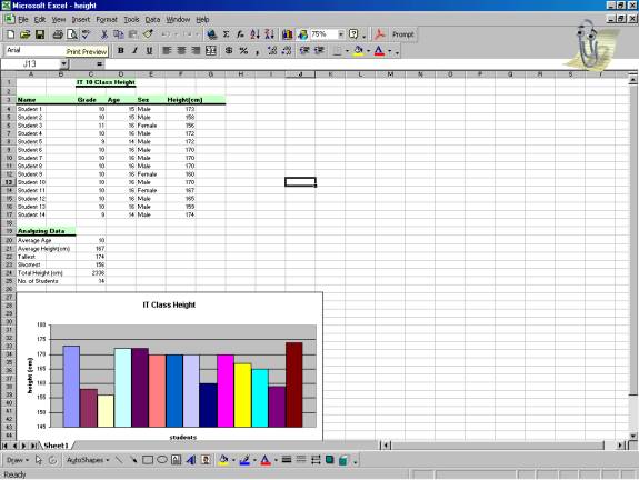
2. cell C1>write in IT 10 Class Height
3. highlight C1, D1>merge and center
4. cell A3>Name>bold
5. cell C3>Grade>bold
6. cell D3>Age>bold
7. cell E3>Sex>bold
8. cell F3>Height (cm)>bold
9. add data of student names, grade, age, sex, height
10. cell??>Average Age>bold
11. cell??>Average Height>bold
12. cell??>Tallest (cm)>bold
13. cell??>Shortest (cm)>bold
14. cell??>Total Height>bold
15. cell??>No. of Students>bold
16. cell??beside Average Age>click =
17. click pulldown>Average
18. click red button spreadsheet>look at the cells needed to calculate this function
19. click red button spreadsheet again
20. type in D4:D??>OK
21. right click>format cell>number>number>decimal places>2>OK
22. repeat same for Average Height, Tallest (Max), Shortest (Min), Sum, and Count A

• Math Operators: * multiplication, / division, + addition, - subtraction

23. file>save as>file name: height>OK>s: drive>it10>it10(your class)(d or f)>your folder>save

Lesson 2

Purpose: students will be able to format the overall look of the spreadsheet, add a graph, and complete a spreadsheet project.

1. Excel>open
2. Kim>it10>it10(your class) (d or f)>your folder>height>open
3. highlight title IT 10 Class Height>format>cell>border>border (top dark line)>style (dark line)
4. format>cell>pattern>choose color>OK
5. highlight height (cm) data>chart wizard
6. standard type: column>next
7. chart source data>highlight data range>series in rows>series>click series 1...2...3...4>change name: student 1...student 2...3...4>next
8. chart options (title: IT 10 Class Height/ Categorie (X) axis: Students/ Value (Y) axis: Height (cm)/ axes: uncheck first box/ gridlines: don't touch/ legend: your choice/ data labels: don't touch/ data table: don't touch)>next
9. chart location>as object in: sheet 1>finish
10. drag to location
11. add clip art or image (1 only)
12. Save
13. Group Project #1: (10 marks)>Create a spreadsheet and graph of the different shoe sizes in your row
    • Title: The Shoe Sizes in my Row
    • Data: Name / Age / Shoe Size
    • Analyzing Data: average shoe size, biggest feet, smallest feet, total inches, no. of students
    • Column Graph: title / legend
    • Clip Art / Image (add 1 only)

Lesson 3

Purpose: students will be able to in plan a project, gather data, analyze data, and create graphs in groups.

Group Project #2: (50 marks)>What percentage of the vehicles in the Sentinel High School parking lot are imports and domestic? Within this data, find the percentage of 2 doors / 4 doors vehicles.

• Title (2 marks)
• Data: total number of vehicles, number of import vehicles, number of domestic vehicles, number of 2 door vehicles, number of 4 door vehicles, percentage of import / domestic, percentage of 2 and 4 door vehicles. (15 marks)
• Analyzing Data: total number of vehicles, number of import vehicles, number of domestic vehicles, number of 2 door vehicles, number of 4 door vehicles, percentage of import / domestic, percentage of 2 and 4 door vehicles. (15 marks)
  
• Graph - 2 graphs (column and bar graphs)- import / domestic and 2 doors / 4 doors: title / legend (10 marks)
• Format: jazz it up! (8 marks)

Click here to see an example.

Lesson 4

Purpose: students will be able to make a hyperlink to another document.

1. Excel>open
2. Kim>it10>it10(your class) (d or f)>your folder>height>open
3. cell above graphs>Conclusion - click here
4. format>cell>border>border (top dark line)>style (dark line)
5. format>cell>pattern>choose color>OK
6. click cell (Conclusion - click here)>hyperlink>type the file or URL>browse>car.doc>OK
7. Save