28/03/6
Adding capacitors in series and in parallel formulae were derived.
In parallel (the same voltage is across each capacitor):
In series:
We then looked at past paper PHY5 and PHY6 questions on capacitors. It was discovered that a few of you need to know a bit more about logs......
22/03/6
We performed an experiment to test how much energy was stored on a capacitor.
A joule meter recorded the electrical energy used in charging a capacitor to various voltages.
Energy used is the area under the graph of voltage against charge.
Energy stored = 1/2 VQ
Substituting in from C=Q/V can give you
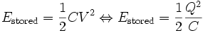

You plotted Energy stored vs. V2 and got a straight line through the origin with a gradient (roughly) equal to the capacitance.
Capacitors in series and parallel next time and that's the lot really.
21/03/6
An assessed practical was completed.
13/03/6
We looked at the analogy between radioactive decay and discharging a capacitor.
The radioactivity of a sample of unstable nuclei is proportional to the number of nuclei present. The rate of change of number of nuclei is equal to the radioactivity. The gradient of an N/t curve is equal to the numerical y values in the second (A/t) at any time.
They all decay with the same basic shape. The rate of discharge in a capacitor is proportional to the amount of charge on it (and hence the voltage across it). The rate of loss of charge on the capacitor is equal to the current flowing at any stage. The gradient of the a Q/t curve is equal to the numerical y values in the second (I/t) at any time.
The mathematics of the 2 phenomena is almost identical.
N (number of nuclei) is analogous to Q (charge)
A (activity) is analogous to I (current)
Lambda (the decay constant) is analogous to 1/RC (inverse of the time constant for the circuit)
Each can be said to have a "half life", although the time constant (Resistance times Capacitance) tends to be used for capacitor discharge. It represents the time taken for the charge, voltage and current to drop to 1/e of it's current value.
"e" is a contant, roughly 2.718 whose size is determined by it being the only number where d/dx (ex) = ex
HW Chapter 12 all practise Qs
8/03/6
RM absent (ill) You started looking at chapter 11 I hope....
7/03/6
We went through the methods (although not the answers) employed in the practical exam. We then charged up some more capacitors, but this time through a variable resistor. We adjusted the variable resistor in such a way as the current stayed the same all the time.
The above graph shows the usual decrease in current over time. The total amount of charge which has flowed is equal to the average current multiplied by the time (Q=It) or the area under the graph. However, it is awkward to calculate the area under the graph without using integration. You may be expected to "count the squares", I hope not.
If, by changing the resistance gradually, the current is kept the same throughout the charging things are much easier.
Q = It, nice and simple.
The capacitor charging graph is exactly the same sort of shape as the graphs which show radioactive decay. Much more on this tomorrow.
HW Qs 10.1, 10.4, 10.5
01/03/6
Onto capacitors. They are essentially a gap in the an electronic circuit built with 2 parallel plates, close enogh together that the electric fields when they are charged can interact.
We charged up a capacitor(eventually) in series with a large resistor and recorded the current every 5 seconds or so.
The current started off at a maximum value, and decreased as the plates became more charged up (making it harder to push charge onto the plates). The shape is the same as that found in radioactive decay graphs, much more on this later.
HW Do qs 9.2-9.5 on capacitor basics please.
28/2/6
A practise practical exam was attempted.
On to capacitors tomorrow.
22/2/6
Equipotentials were discussed in more detail, and a demo of how to measure them using a voltmeter was given. Remember, electrostatic potential is the potential energy per Coulomb of charge at a particular point in a field.
Equipotential lines are perpendicular to field lines at all times.
Between parallel oppositely charged plates, the equipotentials are parallel and equidistant.
As the field gets weaker away from a point charge, the equipotentials get further apart.
21/2/6
Electric charge can be measured by a Coulomb meter. You need to understand the components used to build one. A capacitor and a voltmeter in parallel.
Charge(Coulombs) = Voltage * Capacitance(Farads)
Q = CV
We then looked at the shape of electrostatic field lines.
I was wrong about field shapes between unequal charges.
The shape between 2 oppositely charged plates gets close to a uniform field (where there is no change in field direction or strength.)
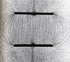
Field lines are parallel here, shown by floating semolina which aligns itself with the field due to an induced dipole being created by the field.
Electric field strength is measured in N/C and is analogous to gravitational field strength. It is not the same as voltage.
Voltage measures the electrical potential energy per Coulomb of charge, not the force. In a uniform field (like between the parallel plates) the field strength is the same at all places, whereas the voltage rises linearly with distance.
So to summarise: electrical force = field strength * charge
electrical potential energy = voltage * charge
Around a point or spherical charge, an oppositely charged particle can perform circular motion, as the electrostatic force can provide the centripetal force required.
This is a rough model of how an atom works....
HW Qs 2-5 from the handout after the field diagrams.
08/2/6
Electrostatic fields follow very similar rules to gravitational fields. The strength of the field diminishes proportionally to 1/r2 as you move away from a point charge. The force between 2 charges increases if you increase either one of the charges in magnitude. This leads to a very similar formula for finding the electrostatic force between 2 charges.
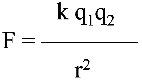
Where k is a constant of proportionality which is analogous to G. It has a value of 9E9N2kg2C-2
It is in fact made up of a combination of further constants making the full formula:
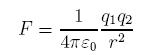
Putting in the relevant signs on the charges gives you a negative number for 2 opposite charges (an attraction) and a positive number for 2 alike charges (repulsion). This differs from gravitation where there is only one type of mass to deal with.
HW Chapter 3 Qs 3.2-3.5 recapping Kepler's 3rd law
07/2/6
Gravitational field lines were discussed. They show the direction of the force which would act on a mass in an area due to the gravitational field. Locally on the the Earth's surface we think of the field as uniform always the same strength and in the same direction (so field lines are parallel).
In actual fact, the field lines always point towards the centre of gravity of the Earth, and so get further apart as you leave the Earth. The further apart the lines are, the weaker the field.
We also taked about the energy required to push masses up in a gravitational field. This is easy in a uniform field (GPE = mgh) but harder when the field is changing.
We'll do something on electrostatics tomorrow.
HW Do the first 2 sheets of the printed handout.
01/2/6
It was delightful to finally see all of you.....
I summarised chapter 1+2 of the new Fields and Synthesis module for those who haven't yet taken it all in.
Basically, simple gravity ideas such as the difference between mass and weight, and the idea that acceleration due to gravity (in m/s2) is the same as gravitational field strength (in N/kg) cover chapter 1.
Chapter 2 introduces the general equation to work out the size of a gravitational force. F = Gm1m2/r2
You must be able to use this to calculate the size of the mutual attraction between 2 masses at a certain distance.
Objects attracted to each other often start to orbit each other. When one mass is vastly larger than the other it looks like the one object is going around the other, which seems stationary. However, the objects actually move around their combined centre of mass.
Sometimes orbits are circular and so all the equations of circular motion from PHY4 can be applied.
We used these to show Kepler's 3rd law (below) is true.
HW First 2 questions from the printed handout sheet (done already by some).
31/1/6
Few people in again. Really not possible to make much progress. Still we saw a little video on Kepler and did a special case derivation of his second and third laws for circular motion.
2nd law: The area swept out by any orbit in a gravitational system is constant
3rd law: T2 is proportional to r3
where T is the period and r the radius of an orbit.
24/1/6
Few people in due to exams. We did a few calculations using F = Gm1m2/r2
24/1/6
Well here you were, back again. (mostly)
We started the new module. Fields, forces and synthesis.
We got going on the fields side of things by looking at gravitational fields. Gravitational forces are easy to calculate if you know the local field strength g.
Force = g * mass (kg)
However, more generally useful is the formula which predicts the gravitational force between any 2 masses.
F = Gm1m2/r2
Where r is the separation of the 2 masses and G is the universal gravitational constant. (6.67E-11)
We did a few calculations using this formula and realised that gravitational forces between masses are generally very small unless the masses involved are large.
Hyperphysics is a great sight for reading around your subject.....
10 + 11 /01/06
Revise revise revise revise!
Good luck all
![]()