
Often in physics, we encounter situations where we have several unknowns. This can happen with motion in two or three dimensions which can produce three or four unknowns. Another situation where we encounter many unknowns is in electronics. In a complex circuit, each circuit branch will have different currents, each dependent on other circuit parameters. It is not unusual to have 6 or more unknowns in a rather simple circuit. To solve these problems, we need to be able to write as many equations as we have unknons, then solve them simultaneously. One way to do this is to solve for one unknown in one equation and substitute that expression into a second equation, thus eliminating one unknown. This works well if you only have two or three unknown, but becomes unwieldy for anything more than that. Often variables can be eliminated by multiplying one equation by a number and then adding the result to another equation. For example, given two equations 4x + 3y = 16 and 6x + y = 10. Using the substitution method, rearranging the second equation will give us y = 10 - 6x. Substitute this into the first equation to eliminate y and get 4x + 3(10 - 6x) = 16. Combine terms to get -14x = -14, or x = 1 and therefore y = 4. Using the adding equations method, if we multiply the second equaiton by -3 we get -18x -3y = -30. Now we can add this to the first equation and get (4x-18x) + (3y-3y) = 16-30 or -14x = -14.
The second mothod of adding equations together underlies the use of matrices to solve systems of equations. We need to devise a method where each equation has only one variable in it, or to put it another way, where one variable has a coefficient of 1 and the others have coefficients of 0. Linear algebra gives us a way to do this using matrices. A matrix is a rectangular array of numbers, and mathematical operations can be performed on these matrices. The matrix is usially designated by a capital letter enclosed in brackets such as [A]. In the language of linear algebra, a one column matrix is referred to as a vector, but we won't worry about that distinction here. When matrices are added together, the terms in corresponding locations are simply added and a new matrix is formed where each term is the sum of the two numbers in the same location in the original matrices. But in matrix multiplication, the columns of the first matrix are multiplied by the rows of the second, so the second matrix must have the same number of rows as the first has columns. Let's see how we can use this in solving equations.
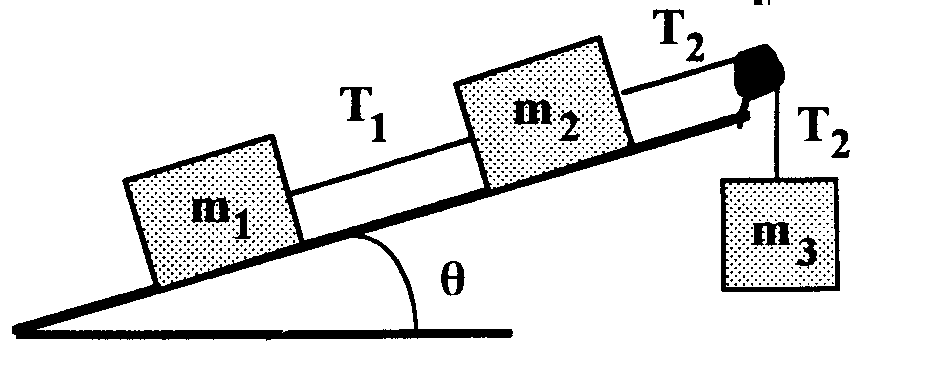
In the figure, two blocks on a frictionless inclined plane which makes an angle of 20 degrees with the horizontal are connected together by a cord and then, by means of a second cord which passes over a massless, frictionless pulley, to a third block which is free to move vertically. The masses of the blocks are m1= 2.00 kg, m2 = 1.00 kg, and m3 = 3.00 kg. When the system is released, block 3 will accelerate towards the floor with blocks 1 and 2 accelerating up the ramp. The problem here is to find the tension in the two ropes and the acceleration of the system. A traditional method would involve isolating parts of the system and applying Newton's 2nd law to each part. Another method would be to write the 2nd law equation for each block and solve simultaneously. This will give three equations in three unknowns, T1, T2, and a. The three equations are:
for block 3: m3g - T2 = m3a
for block 2: T2 - T1 - m2g(sin 20°) = m2a
for block 1: T1 - m1g(sin 20°) = m1a
Plugging in the values for the masses, using 10 m/s2 for g, and dropping units we get:
eq 1 for block 1: T1 - 6.84 = 2.00a
eq 2 for block 2: T2 - T1- 3.42 = 1.00a
eq 3for block 3: 30.0 - T2 = 3.00a
Now in order to use matrices with these equations we need to rearrange them. Put all of the terms with unknowns on the left side of the equation, putting the terms in the same order in all three equations.
| T1 term | T2 term | a term | equals | numbers |
| 1T1 | +0T2 | -2.00a | = | 6.84 |
| -1T1 | +1T2 | -1.00a | = | 3.42 |
| 0T1 | +1T2 | +3.00a | = | 30.0 |
Notice that I included coefficients of 0 and 1 even though these are not often written in normal equations. I also changed the signs on equation 3 (multiplied both sides by -1). Take a look at the terms on the left side of the three equations. Remembering what was said above about multiplying matrices, these terms could be the product of two matrices, matrix [A] being a 3 x 3 matrix of the coefficients of the unknowns and matrix [B] being the three unknowns themselves.
Matrix [A] =
| 1 | 0 | -2.00 |
| -1 | 1 | -1.00 |
| 0 | 1 | 3.00 |
And Matrix [B] =
| T1 |
| T2 |
| a |
The product of [A][B] gives us the left side of the three equations. That must mean that this product also gives us a third matrix [C] composed of the three numbers on the right side of the equations.
So matrix [C] =
| 6.84 |
| 3.42 |
| 30.0 |
And we now have the matrix equation [A][B] = [C]. Now when working with matrices, we have to follow special rules for mathematical operations, but often they are analogous to ordinary math. One of these is the inverse matrix which corresponds to the reciprocal of a number. We know that when a number and its reciprocal are multiplied together, the answer is one. When a matrix and its inverse are multiplied together a third matrix called the identity matrix results. So when we multiply [A][A]-1 we get the identity matrix:
| 1 | 0 | 0 |
| 0 | 1 | 0 |
| 0 | 0 | 1 |
Finding the value of this inverse matrix can be a difficult process but fortunately the graphing calculators will do the job for us. So to find the solution to our problem, we need to find the numbers that go with our matrix [B] of unknowns. If we multiply both sides of the matrix equation [A][B] = [C] by [A]-1, we get [B] = [A]-1[C]. In other words the solutions for our three unknowns can be found by the product of the inverse coefficients matrix and the number matrix.
Each model of graphing calculator is a little different in the menus and keystrokes, so you should refer to your owners manual for more complete instructions. In general here are the steps to set up a matrix. First you must select a name (letter) for the matrix. On the TI 83+ which I have, use 2nd, MATRX, scroll to an unused letter and go to the EDIT command at the top. You must now enter the dimensions of your matrix, the number of rows and columns. The default is 1 x 1. For our matrix [A], we need a 3 x 3 matrix. When the dimensions are set up, the cursor moves to the first item in the matrix so that values may be entered. The values are all zero by default until changed. When all values are entered, quit the operation and repeat for other matrices. For [B] and [C] the dimensions are 3 x 1, three rows and 1 column and matrix [B] has no values to enter at this time. Once the matrices are in the calculator memory, you can do math operations on them by going to the matrix list and selecting the matrix you need. To work the problem [B] = [A]-1[C] on the TI 83+, go 2nd, MATRX, select [A], then the x-1key; now go 2nd, MATRX and select [C]; now store the results in [B] by going STO, 2nd, MATRX, select [B]. You'll find the answers will be T1 = 13.42 N, T2 = 20.13 N, and a = 3.29 m/s2. Since the matrix does not hold units, you must do the unit analysis separately.
Although this fairly simple problem could be solved without the use of matrices, it does make the problem even easier. More complicated situations with more unknowns become an algebraic nightmares that can be greatly simplified by the power of matrices.