Filtered-U Recursive LMS (RLMS) Algorithm

    The adaptive infinite impulse response (IIR) filter  was proposed by Eriksson  for use in active noise control. This approach considers the acoustic feedback as a part of the whole acoustic plant, and the poles introduced by the acoustic feedback are removed by the poles of the adaptive IIR filter. This control system dynamically tracks changes in the secondary and feedback paths during cancellation operations. The IIR structure has the ability to model transfer functions directly with poles and zeros. Although there are various adaptive IIR algorithms that can be used, the recursive LMS (RLMS) algorithm developed by Feintuch is selected here for reasons of computational simplicity.

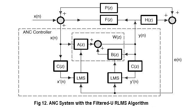
    The RLMS algorithm must also be modified to compensate for the transfer function of the secondary and feedback paths. A block diagram of an ANC system using an adaptive IIR filter is shown in Figure 12, where y(n) is the output signal of IIR filter computed by:

y(n) = a   (n) * x(n) + b  (n) * y(n - 1)

             N-1                                       M
        =  sum {  a i (n) * x(n - i)  } +  sum  {  b j (n) * y(n -j)  }                                                                                         (1)
            i = 0                                      j = 1

where:
a (n) = [a0 (n)   a1  (n) … aN (n)]    is the weight vector of A(z) at time n

b (n) = [b0  (n)   b1  (n) … bM-1 (n)]    is the weight vector of B(z) at time n

y (n - 1) = [y (n - 1)  y (n - 2) … y (n - M)]    is the signal vector containing output
                                                                          feedback with one delay
N = order of A(z)
M = order of B(z)
 

    The filtered-U RLMS algorithm can be expressed by two vector equations for adaptive filters A(z) and B(z) as follows:

a(n + 1) = a(n) - mu * e(n) * x’(n)                                                                                                                                     (2)
and

b(n + 1) = b(n) - mu * e(n) * y’(n -1)                                                                                                                                (3)
where:

y’(n - 1) = [y’(n - 1)   y’(n - 2) …. y’(n -M)]                                                                                                                    (4)
and

                M
y' (n) =   sum    {  c i * y(n -j)   }                                                                                                                                      (5)
              j = 1

is the filtered y(n) from C(z), and x’(n) is the filtered version of x(n).
 

    After both A(z) and B(z) converge, the measured residual error signal e(n) is equal to zero. Now:

W(z) =     A(z) / (1- B(z) )    =     -P(z) / ( H(z) - P(z)*F(z) )                                                                                           (6)
 

    Given the complexities and pole-zero structure of P(z), H(z), and F(z), the convergence of A(z) and B(z) cannot be generalized. The optimum solutions A*(z) and B*(z) are not unique; however, the algorithm will converge to a solution that minimizes the residual error signal e(n). Based on equation (4.6.6), one possible set of solutions is:

A*(z) =  -P(z)/H(z)                                                                                                                                                           (7)
 
and

B*(z) =  P(z) * F(z) / H(z)                                                                                                                                                (8)
 

    Therefore, it is reasonable to use a higher order for B(z) than for A(z).

    The system performs the off-line modeling to estimate the secondary-path transfer function using the algorithm summarized in the section on the FXLMS algorithm. After the off-line modeling, the ANC system is operated in noise cancellation mode. The detailed algorithm, shown in Figure 12, is summarized as follows:

1. Input the reference signal x(n) and the error signal e(n) from the input ports.

2. Compute the antinoise y(n):

                 N-1                                         J
    y(n) =  sum  {  a i (n) * x(n - i)  } +  sum  {  b j (n) * y(n - j) }                                                                                     (9)
                i = 0                                      j = 1

    where N is the order of the filter A(z) and J is the order of the filter B(z).

3. Output the antinoise y(n) to the output port to drive the canceling speaker.

4. Perform the filtered-U operation:

                 M-1
    x’(n) =  sum    {  c i *  x(n - i) }                                                                                                                                  (10)
                 i = 0

    and

                 M-1
   y’(n) =   sum     {  c i * y(n - i - 1)  }
                 i = 0

    where M is the order of the filter C(z).

5. Update the coefficients of the adaptive filters A(z) and B(z) using the filtered-U RLMS
    algorithm:

    a i (n + 1) =  a i (n) + mu * e(n) * x’(n - i),          i = 0, 1,..., N - 1                                                                             (11)

    and
 
    b j (n + 1) =  b j (n) + mu * e(n) * y’(n - j),           j = 1, 2,..., J                                                                                   (12)

6. Repeat the algorithm for the next iteration.