The FXLMS algorithm
Algorithms for Broadband Feedforward ANC Systems
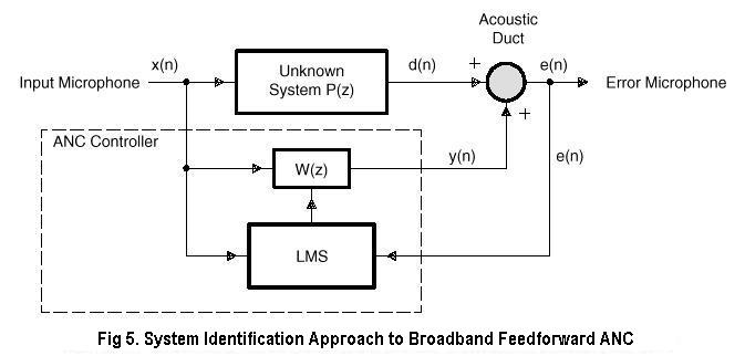
Broadband active noise control can be described in a system identification framework, as shown in Figure 5. Using a digital frequency-domain representation of the problem, the ideal active noise control system uses an adaptive filter W(z) to estimate the response of an unknown primary acoustic path P(z) between the reference input sensor and the error sensor. The z-transform of e(n) can be expressed as:
E(z) = D(z) + Y(z) = X(z) * [P(z) + W(z)] (1)
where,
E(z) is the error signal,
X(z) is the input signal,
Y(z) is the adaptive filter output.
After the adaptive filter W(z) has converged, E(z) = 0. Hence equation (1) becomes:
W(z) = - P(z) (2)
which implies that:
y(n) = - d(n) (3)
Therefore, the adaptive filter output y(n) has the
same amplitude but is 180° out of phase with the primary noise d(n).
When d(n) and y(n) are acoustically combined, the residual error becomes
zero, resulting in cancellation of both sounds based on the principle
of superposition.
Secondary-Path Effects
The error signal e(n) is measured at the error microphone
downstream of the canceling speaker. The summing junction in Figure 5 represents
the acoustical environment between the canceling speaker and the error
microphone, where the primary noise d(n) is combined with the antinoise
y(n) output from the adaptive filter. The antinoise signal can be modified
by the secondary-path function H(z) in the acoustic channel from y(n) to
e(n), just as the primary noise is modified by the primary path P(z) from
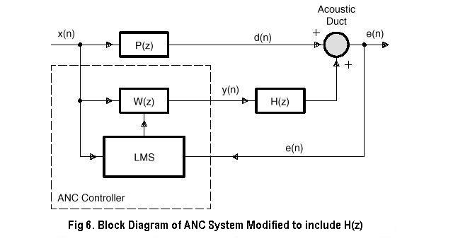
the noise source to the error sensor. Therefore, it is necessary to compensate
for H(z). A more detailed block diagram of an active noise control system
that includes the secondary path H(z) is shown in Figure 6.
From Figure 6, the z-transform of error signal e(n) is:
E(z) = X(z) * P(z) + X(z) * W(z) * H(z) (4)
Assuming that W(z) has sufficient order, after the convergence of the adaptive filter, the residual error is zero (that is, E(z) = 0). This result requires W(z) to be:
W(z) = - P(z) / H(z)
(5)
to realize the optimal transfer function.
Thus, the adaptive filter W(z) has to model the primary path P(z) and inversely model the secondary path H(z). However, it is impossible to invert the inherent delay caused by H(z) if the primary path P(z) does not contain a delay of at least equal length. This is the overall limiting causality constraint in broadband feedforward control systems.
Furthermore, from equation (5), the control system
is unstable if there is a frequency w such that H(w) = 0. Also, the control
system is ineffective if there is a frequency w where P(w) = 0, (that is,
a zero in the primary path causes an unobservable control frequency). Therefore,
the characteristics of the secondary path H(z) have significant effects
on the performance of an ANC system.
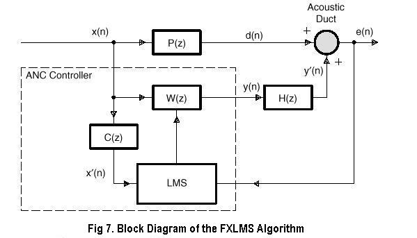
Filtered-X Least-Mean-Square (FXLMS) Algorithm
To account for the effects of the secondary-path
transfer function H (z), the conventional least-mean-square (LMS) algorithm
needs to be modified. To ensure convergence of the algorithm, the input
to the error correlator is filtered by a secondary-path estimate C(z).
This results in the filtered-X LMS (FXLMS) algorithm developed by Morgan.
Burgess has suggested using this FXLMS algorithm to compensate for the
effects of the secondary path in ANC applications.
The FXLMS algorithm is illustrated in Figure 7, where the output y(n) is computed as:
N
y(n) = Sum { w i (n) * x(n - i) }
(6)
i = 0
where,
w i (n) is the ith coefficient of the FIR filter W(z)
at time n , and
x(n) is the reference signal vector at time n.
The FXLMS algorithm can be expressed as:
w(n + 1) = w(n) - mu * e(n) * x(n) * h(n) (7)
where mu is the step size of the algorithm that determines the stability and convergence of the algorithm and h(n) is the impulse response of H(z). Therefore, the input vector x(n) is filtered by H(z) before updating the weight vector. However, in practical applications, H(z) is unknown and must be estimated by the filter, C(z). Therefore:
w i (n + 1) = w i ( n) - mu * e(n) * x(n - i) i = 0, 1 ,..., N - 1 (8)
and:
w(n + 1) = w(n) - mu * e(n) * x(n) (9)
where:
M
x(n) = sum { C i * x(n - i) }
(10)
i = 0
is the vector for the filtered version of reference input x(n) that is written as:
x(n) = [x(n) x(n - 1) .. x(n - N + 1)] (11)
and:
C = [ C0 C1 . CM ] (12)
is the coefficient vector of the secondary-path estimate, C(z).
When this algorithm is implemented, the convergence of the filter can be achieved much more quickly than theory suggests, and the algorithm appears to be very tolerant of errors made in the estimation of the secondary path H(z) by the filter C(z). As shown by Morgan , the algorithm still converges with nearly 90° of phase error between C(z) and H(z).
It is important that in equation (7), a minus sign is used for ANC applications instead of a plus sign as in a conventional LMS algorithm. This is because the error signal in an ANC system is e(n) = d(n) + y(n), due to the fact that the residual error e(n) is the result of acoustic superposition (addition) instead of electrical subtraction.
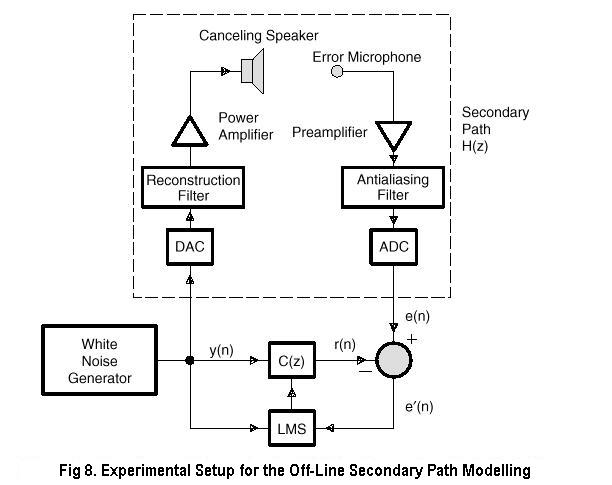
The transfer function H(z) is unknown and is time-varying
due to effects such as aging of the loudspeaker, changes in temperature,
and air flow in the secondary path. Thus, several on-line modeling techniques
were developed by Eriksson. Assuming the characteristics of H(z) are unknown
but time-invariant, an off-line modeling technique can be used to estimate
H(z) during a training stage. At the end of training, the estimated model
C(z) is fixed and used for active noise control. The experimental setup
for the direct off-line system modeling is shown in Figure 8, where an
uncorrelated white noise is internally generated by the DSP.
1. Generate a sample of white noise y(n).
2. Input the secondary-path response e(n) from the error microphone.
3. Compute the response of the adaptive model r(n):
M
r(n) = sum {
C i ( n) * y(n - i) }
(13)
i = 0
where C i (n) is the ith
coefficient of the adaptive filter C(z) at time n and M is the order of
filter.
4. Compute the difference:
e(n) = e(n) - r(n)
(14)
5. Update the coefficients of the adaptive filter C(z) using the LMS algorithm:
C i (n + 1) = C i (n) + mu * e(n)
* y(n - i),
i = 0, 1,..., M - 1
(15)
where mu is the step size that must
satisfy the following stability condition:
0 < mu < 1 /
( M * autocorrelation of i/p (0) )
(16)
6. Repeat the procedure for about 10 seconds. Save the coefficients
of the adaptive filter C(z) and use them in the
following noise cancellation mode.
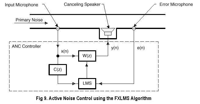
After the off-line modeling is completed, the system
is operated in the active noise cancellation mode. The algorithm is illustrated
in Figure 9, and the procedure of on-line noise control is summarized after
the figure on the following page.
1. Input the reference signal x(n) (from the input microphone) and the error signal e(n) (from the error microphone) from
2. Compute the antinoise y(n):
N
y(n) = sum
{ w i ( n) * x(n - i) }
(17)
i = 0
where w i ( n) is the ith coefficient
of the adaptive filter W(z) at time n and N is the
order of filter W(z).
3. Output the antinoise y(n) to the output port to drive the canceling loudspeaker.
4. Compute the filtered-X version of x(n):
M
x(n) = sum
{ C i * x(n - i) }
(18)
i = 0
5. Update the coefficients of adaptive filter W(z) using the FXLMS algorithm:
w i (n + 1) = w i (n) - mu * e(n) *
x(n - i),
i = 0, 1,..., N - 1
(19)
6. Repeat the procedure for the next iteration. Note that the total
number of memory locations required for this algorithm
is 2(N + M) plus some parameters.