FBFXLMS algorithm

Acoustic Feedback Effects and Solutions (FBFXLMS Algorithm)

Referring again to the simple system shown in Figure 2, the antinoise output to the loudspeaker not only cancels acoustic noise downstream, but unfortunately, it also radiates upstream to the input microphone, resulting in a contaminated reference input x(n). This acoustic feedback introduces a feedback loop or poles in the response of the model and results in potential instability in the control system.

This problem has been intensively studied in active noise and vibration control literature. Solutions such as the following have been proposed:

1. Using directional microphones and speakers. (This has a limitation in that directional arrays are usually highly
dependent on the spacing of the array elements and are directional over only a relatively narrow frequency range.)

2. Using fixed compensating signals (generated from the compensating filter whose coefficients are determined off-line
by using a training signal) to cancel the effects of the acoustic feedback.

3. Using a second off-line adaptive filter in parallel with the feedback path

4. Using an adaptive IIR filter

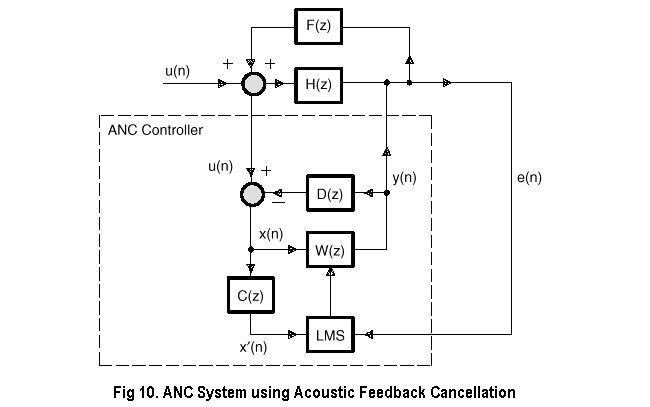
This report examines methods 2 and 4. An adaptive feedforward controller with feedback compensation is shown in Figure 10. The filter D(z) is an estimate of the feedback path F(z) from the adaptive filter output y(n) to the output of the reference input microphone u(n). Filter D(z) removes the acoustic feedback from the reference sensor input; the filter C(z) compensates the secondary-path transfer function H(z) in the FXLMS algorithm. Removal of the acoustic feedback from the reference input adds a considerable margin of stability to the system if the model D(z) is accurate. The models C(z) and D(z) can be estimated simultaneously by an off-line modeling technique using an internally generated white noise.

    The expressions for the antinoise y(n), filtered-X signal x’(n), and the adaptation equation for the FBFXLMS algorithm are the same as that for the FXLMS ANC system, except that x(n) in FBFXLMS algorithm is a feedback-free signal that can be expressed as:
                        L
x(n) = u(n) -   sum   { d i * y(n - i) }                                                                                                                              (1)
                      i = 0
where,
u(n) is the signal from input microphone,
d i is the ‘i’th coefficient of D(z), and
L is the order of D(z).

In the case of a perfect model of the feedback path (that is, D(z) = F(z)), the acoustic feedback is completely canceled by D(z). The function of D(z) is similar to the acoustic echo cancellation that is used in teleconferencing applications.

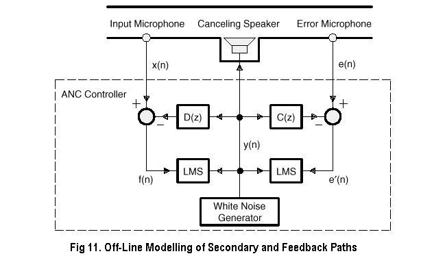
The system performs the off-line modeling first to estimate the secondary-path transfer function H(z) from the canceling speaker to the error microphone and the feedback path transfer function F(z) from the canceling speaker to the input microphone. The off-line modeling algorithm is illustrated in Figure 11 and the procedure is summarized following the figure.

1. a. Generate a white noise sample y(n).
    b. Output this excitation signal y(n) to drive the canceling loudspeaker.
    c. Send y(n) to the adaptive filters C(z) and D(z).
    d. Send y(n) to the LMS algorithm for updating C(z) and D(z).

2. Input x(n) from the input microphone and e(n) from the error microphone.

3. Compute e’(n) and f(n):

                             M-1
     e’(n) = e(n) -   sum     { c i (n) * y(n - i) }                                                                                                                (2)
                             i = 0

and

                            L-1
     f(n) = x(n) -   sum    { d j (n) * y(n - j) }                                                                                                                    (3)
                           j = 0

4. Update the coefficients of the adaptive filters C(z) and D(z) using the LMS algorithm:

c i (n + 1) = c i (n) + mu * e’(n) * y(n - i), i = 0, 1,..., M - 1 (4)

and

d j (n + 1) = d j (n) + mu * f(n) * y(n - j), j = 0, 1,..., L - 1 (5)

5. Repeat the off-line modeling for about 10 seconds. Save the coefficients of adaptive
filters C(z) and D(z) and use them in the following active noise cancellation mode.

After the off-line modeling, the ANC system is operated in active noise cancellation mode. The algorithm is summarized as follows:

1. Input u(n) and e(n) from the input ports.

2. Compute the feedback-free reference input x(n):

                           L-1
    x(n) = u(n) -   sum     { d j * y(n - j) }                                                                                                                         (6)
                          j = 0

3. Compute the antinoise y(n):

                 N-1
    y(n) =   sum    { w i (n) * x(n - i) }                                                                                                                             (7)
                i = 0

    where
    w i (n) is the ‘i’th coefficient of the adaptive filter W(z) at time n ,and
    N is the order of filter W(z).

4. Output the antinoise y(n) to the output port to drive the canceling loudspeaker.

5. Compute the filtered-X version of x(n):

                   M
     x’(n) = sum     { c i * x(n - i) }                                                                                                                                 (8)
                  i = 0

6. Update the coefficients of adaptive filter W(z) using the following FXLMS algorithm:

w i (n + 1) = w i (n) + mu * e(n) * x’(n - i), i = 0, 1,..., N - 1 (9)

5. Repeat the algorithm for the next iteration. Note that the total number of memory locations required in this algorithm
is 2(N + M + L) plus some parameters.