Results
Traffic (Trail-use Intensity)
The data revealed that CAPH and the TRC had the highest and lowest traffic levels, respectively (Figure 3.2). The two lodges with the highest values were also those that have been established the longest.
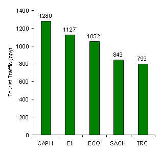
Figure 3.2. Tourist traffic (trail-use intensity) measured in terms of average number of people per year (ppyr) who used the tourist transects over a 5 year period (1994-1998 inclusive). [This data is not equal to total annual tourist arrivals at each lodge.]
Habitat and Fruit Resources
Five genera of fruiting tree dominated the plants under investigation, and accounted for between 70-90% of the samples (in decreasing order of abundance): Iriartea*, Astrocaryum*, Pseudolmedia, Scheelea*, and Ficus* (Figures 3.4-3.8), 4 of which (*) also provide keystone fruit resources for many mammals. The overall density of fruiting trees was highest at the TRC (86 trees/ha) and lowest at CAPH (39 trees/ha)(Figure 3.3).
Iriartea
This palm was by far the most consistently abundant genera at each lodge, making up between 41-82% of the trees under investigation. T-tests revealed that only at the EI was there a significant difference in the density of this palm between T and C (T = 28 trees/ha; C = 21 trees/ha; t = 2.16, p < 0.05) (Figure 3.4). The lodges with the highest and lowest average density were TRC (69 trees/ha) and CAPH (14 trees/ha), respectively. Further t-tests revealed that the abundance of this palm was significantly greater at the TRC than at any other lodge.
Scheelea
T-tests revealed that at the EI, ECO and TRC there was a significant difference in the density of this palm between T and C, however there was no consistent trend either way to suggest that tourism was in any way responsible for the difference (Figure 3.5). The lodges with the highest and lowest average density were ECO (9 trees/ha) and TRC (0.5 trees/ha), respectively. The TRC had a significantly lower density of this palm than any other lodge, although the average density was not significantly different between the other four lodges.
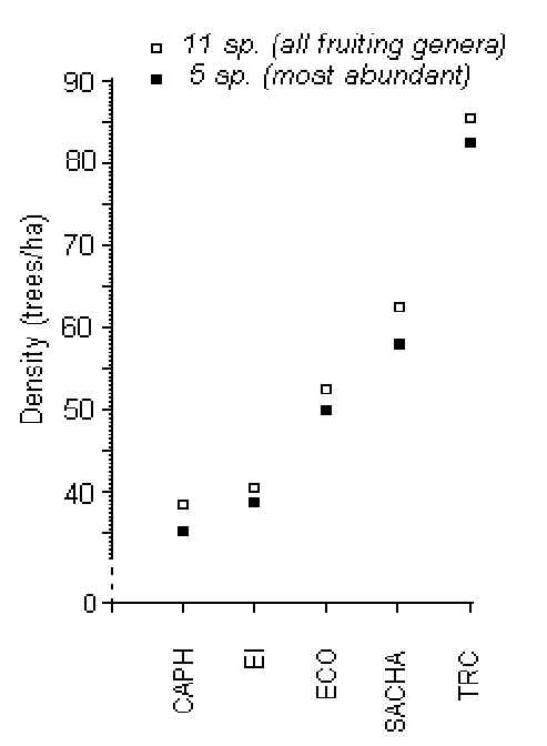
Figure 3.3. Average cumulative density from lodge to lodge of all 11 fruiting genera (white squares) and the 5 most abundant genera (black squares).
Astrocaryum
T-tests revealed that at CAPH, ECO, SACHA and TRC there was a significant difference in density between T and C, however there was no indication that tourism had any role in this (Figure 3.6). The lodges with the highest and lowest average density were ECO (13 trees/ha) and EI (2 trees/ha), respectively. The EI had a significantly lower density than any other lodge. The average density was not significantly different between the other 4 lodges.
Pseudolmedia
T-tests revealed that at CAPH, SACHA and TRC there was a significant difference in density between T and C, however there was no indication that tourism had any role in this (Figure 3.7). The lodges with the highest and lowest average density were ECO (8 trees/ha) and TRC (4 trees/ha), respectively. The density between ECO and SACHA was not significantly different although they both had significantly higher densities that the other three lodges.
Ficus
T-tests revealed that only at ECO was there a significant difference in density between T and C (T = 3.4 trees/ha; C = 2.2 trees/ha; t = 2.19, p < 0.03)(Figure 3.8). The lodges with the highest and lowest average density were ECO (2.8 trees/ha) and EI (1.8 trees/ha), respectively, although as a whole there were no significant differences in density between lodges.
Guadua
Bamboo was completely absent from the two lodges located along the Madre de Dios River (CAPH and ECO). It was most common along the Tambopata River at SACHA where it was more abundant along C than along T (Figure 3.9). At EI the average relative density was lower than at the other two lodges located along the Tambopata River, which in turn were found to be not significantly different from one another.
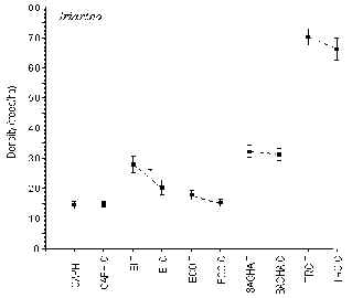
Figure 3.4. Density of the pona palm (Iriartea); * significant difference between T and C.
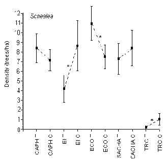
Figure 3.5. Density of the shebon palm (Scheelea); * significant difference between T and C.
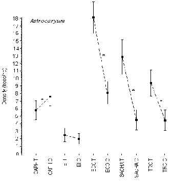
Figure 3.6. Density of the huicunguo palm (Astrocaryum); * significant difference between T and C.
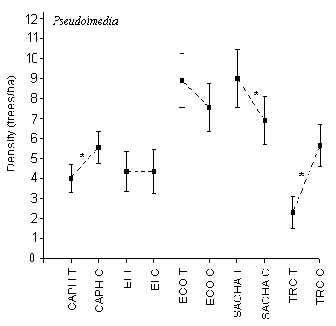
Figure 3.7. Density of the chimicua tree (Pseudolmedia); * significant difference between T and C.
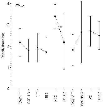
Figure 3.8. Density of the fig tree (Ficus); * significant difference between T and C.
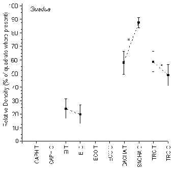
Figure 3.9. Relative density of Bamboo (Guadua); * significant difference between T and C.
A multivariate hierarchical cluster analysis revealed that lodges which are geographically close to one another are more similar in terms of the 13 genera studied (Figure 3.10) than those far apart, although in the majority of cases more than 50% of the available data is dominated by just one genera (Iriartea). The major indicator genera which can explain the majority of the cluster pattern are: Iriartea, Pseudolmedia, and Guadua. The grouping together of the 4 lodges most closely associated with human colonisation and the large discrepancy between these and the TRC may well be likely to historical anthropomorphic pressures on these genera, particularly the palms which are frequently used by the native and non-native peoples of the area. Iriartea for instance, which is responsible for the majority of the similarity between the 4 lodges is a common construction material and is also felled frequently to provide breeding grounds for beetle larvae which are a local delicacy. Climate may also be playing a role in the observed abundance patterns as it is known that the TRC receives more annual precipitation than the other lodges.
ECO ---+
+-----+
CAPH ---+ +
+-----------------------------------------+
EI -----+ + +
+---+ +
SACHA-----+ +----------
+
TRC ---------------------------------------------------+
Figure 3.10. Hierarchical cluster analysis of lodges based on the abundance of 13 plant genera.
Hunting Pressure
Data on spent shotgun cartridges found and encounters with local people carrying shotguns, showed that hunters are active at 3 lodges (SACHA, CAPH and ECO), however those with the highest hunting indices by far were SACHA and CAPH (Table 3.2). A Spearman correlation coefficient was calculated to analyse the relationship between hunting index and the relative abundance of five species frequently sought by hunters in Madre de Dios. The result was significantly negative (Spearman = -0.87, p < 0.05) (Table 3.3). One might have expected that EI be heavily affected from this activity due to its location near the native Ese’eja community of Infierno and the community of La Torre, however it appears that over the last 20 years or so these communities have largely respected the "reserve" status of the land used for tourism and do not now hunt within it. Data collected on the abundance of the Spix�s guan (P. jacquacu) also strongly suggests that hunting is very prevalent at CAPH and SACHA (Figure 3.11). Furthermore, the conclusions of Ascorra (1997) serve to reinforce these results.
Table 3.2. Hunting pressure variables at each lodge.
| Lodge | No. of people encountered with rifles |
Cartridges found along trails (1=Yes, 0=No) |
Hunting Index |
Distance travelled (km) |
| SACHA | 5 |
1 |
6 |
296 |
| CAPH | 4 |
1 |
5 |
315 |
| ECO | 1 |
1 |
2 |
310 |
| EI | 0 |
0 |
0 |
172 |
| TRC | 0 |
0 |
0 |
181 |
Table 3.3. Spearman Rank Correlation Coefficient a lodge’s hunting index and the relative abundance of 5 species frequently sought after by hunters in Madre de Dios (Collared Peccary, Brazilian Tapir, Red Howler, Brown capuchin, Red Brocket Deer). Relative abundance was transformed using the following formula Sqrt(abundance+1).
| Lodge | Hunting Index |
Mammal Abundance Score |
Spearman Corr. Coef. |
| SACHA | 6 |
5.160 |
- 0.87 * |
| CAPH | 5 |
5.102 |
. |
| ECO | 2 |
5.357 |
. |
| EI | 0 |
5.378 |
. |
| TRC | 0 |
5.725 |
. |
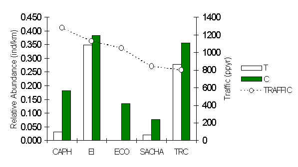
Figure 3.11. Relative abundance (individuals/km walked) of the Spix�s Guan (Penelope jacquacu).
Transect Sample Effort
Sampling effort, measured in terms of diurnal kilometres walked, along T and C transects at any lodge was very similar (Table 3.4). However, there were substantial differences in overall effort between lodges, the greatest extreme being 172 km (EI) versus 315 km (CAPH), a difference of 45%. This was due to a combination of factors; varying total transect lengths between lodges (EI had the lowest total) and the fact that TRC was only visited on five occasions and not the planned six. Overall, the total sample effort for the study was 1,274 km which is far more than any other study of its kind. The average speed of travel during transect censusing was 1.11 km/hr, which is close to the desired speed of 1 km/hr.
Table 3.4. Total number of kilometres sampled at each lodge.
| Lodge | Tourist Transects (km) |
Control Transects (km) |
Total (km) |
| CAPH | 156 |
159 |
315 |
| EI | 86 |
86 |
172 |
| ECO | 155 |
155 |
310 |
| SACHA | 151 |
145 |
296 |
| TRC | 97 |
84 |
181 |
| Total | 645 |
629 |
1,274 |
Species Richness (No. of Species)
Between 21-27 species of mammal were recorded visually and by track data at each lodge, for a total of 31 species, during transect censuses and at opportunistic encounters at other times (Figure 3.12). There was no statistical difference in species richness between T and C transects at any lodge. However, richness was found to be significantly negatively correlated with hunting pressure (Spearman = –0.90, p < 0.05). Both of these results suggest that tourist traffic on its own has little effect on species richness.
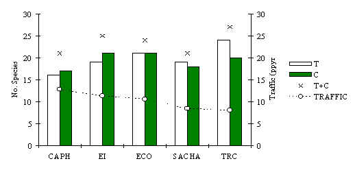 Figure 3.12. Species richness at each lodge,
determined from visual observations and track data collected during transect surveys and
opportunistic encounters.
Figure 3.12. Species richness at each lodge,
determined from visual observations and track data collected during transect surveys and
opportunistic encounters.
Group Size
On many occasions it was impossible to accurately count groups because they were spread so sparsely over a relatively large area, however when a group was located feeding in a tree or travelling rapidly in linear formation over a transect it was possible to count them with more accuracy. Estimates of average group size per species were calculated from data on complete counts of groups when encountered during strict transect surveys and during opportunistic encounters along the transects at other times.
The species with the largest group size was the squirrel monkey (Saimiri boliviensis) which on one occasion reached 85 individuals (at SACHA). T-tests revealed that there was no significant variation in group size for any species between T and C transects at any lodge. However, further tests using pooled data from each lodge revealed that group sizes for the saddleback tamarin (Saguinus fuscicollis) (Figure 3.13; Table 3.5) and brown capuchins (Cebus apella) (Figure 3.14; Table 3.6) varied significantly between some lodges. Pearson rank correlation coefficients revealed that tamarin group size was significantly positively correlated with traffic (Pearson = +0.92, p < 0.05), whilst that of the capuchin was significantly negatively correlated with hunting pressure (Pearson = -0.88, p < 0.05). Overall, average group sizes calculated for a number of species are very similar to those found in other studies in Madre de Dios (Janzen et al. 1980, Freese et al. 1982, Kiltie 1983, Terborgh 1983, Ascorra 1997) (Table 3.7).
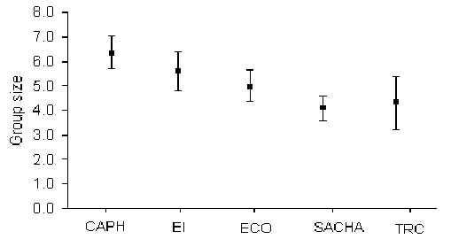
Figure 3.13. Group size variation between lodges for the saddleback tamarin (S. fuscicollis).
Table 3.5. Probability values derived from t-tests of tamarin group sizes. * p < 0.05, ** p < 0.01.
| . | CAPH |
EI |
ECO |
SACHA |
| EI | 0.06 |
. | . | . |
| ECO | 0.00** |
0.15 |
. | . |
| SACHA | 0.00** |
0.00** |
0.02* |
. |
| TRC | 0.00** |
0.04* |
0.15 |
0.36 |
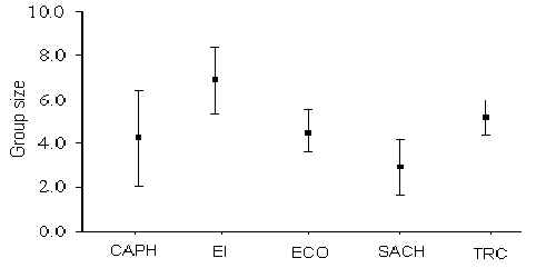
Figure 3.14. Group size variation between lodges for the brown capuchin (C. apella).
Table 3.6. Probability values derived from t-tests of brown capuchin group sizes. * p < 0.05, ** p < 0.01.
CAPH |
EI |
ECO |
SACHA |
|
| EI | 0.05* |
. | . | . |
| ECO | 0.41 |
0.01* |
. | . |
| SACHA | 0.16 |
0.00** |
0.02* |
. |
| TRC | 0.25 |
0.03* |
0.18 |
0.00* |
Table 3.7. Summary of group size estimation using data from complete counts of identifiable conspecific and mixed species groups at all lodges. Other Studies: 1 Freese et al. (1982), 2 Kiltie et al. (1983), 3Warner (1999).
| Species | . | Group Size | . | . | 95% CI |
Group Size |
||
| Common Name | Scientific Name | N |
Min. |
Max. |
Ave |
. | . | |
| Southern Tamandua | T. tetradactyla | 15 |
1 |
2 |
1.10 |
+/- 0.10 |
. | |
| Saddleback Tamarin | S. fuscicollis | 288 |
1 |
16 |
5.40 |
+/- 2.20 |
6, 7 (1, 3) |
|
| Squirrel Monkey | S. boliviensis | 57 |
1 |
85 |
28.60 |
+/- 5.32 |
40, 18 (1, 3) |
|
| Dusky titi Monkey | C. brunneus | 44 |
1 |
6 |
2.70 |
+/- 1.90 |
3, 3 (1, 3) |
|
| Red Howler | A. seniculus | 54 |
1 |
10 |
4.00 |
+/- 0.60 |
5 (1) |
|
| White-fronted Capuchin | C. albifrons | 8 |
1 |
32 |
12.5 |
+/- 8.30 |
. | |
| Brown capuchin | C. apella | 109 |
1 |
12 |
4.70 |
+/- 1.10 |
10, 6 (1, 3) |
|
| Black Spider Monkey | A. paniscus | 34 |
1 |
16 |
5.20 |
+/- 1.30 |
7 (1) |
|
| South American Coati | N. nasua | 25 |
1 |
15 |
5.40 |
+/- 1.80 |
. | |
| Collared Peccary | T. tajacu | 75 |
1 |
9 |
2.00 |
+/- 0.30 |
2 (2) |
|
| Bolivian Squirrel | S. ignitus | 118 |
1 |
6 |
1.14 |
+/- 0.10 |
. | |
| Southern Amazon Red Squirrel | S. spadiceus | 672 |
1 |
5 |
1.15 |
+/- 0.04 |
. | |
| Brown Agouti | D. variegata | 364 |
1 |
3 |
1.10 |
+/- 0.03 |
. | |
Mammal Abundance
After 23 months of censuses along T and C transects we visually observed a total of 26 species and took data on 1,328 mammal groups, which on equated to 4,568 individual animals. Encounter rates for each species, in terms of groups and individuals encountered per km walked are summarised in Tables 3.8-3.10. The three most often encountered species were the southern amazon red squirrel (Sciurus spadiceus) with 516 encounters, saddleback tamarin (S. fuscicollis) with 176 encounters, and the brown agouti, with 169 encounters. Five species were observed on only one occasion while 15 species were observed on 10 seperate occasions or more.
Table 3.8. Number of visual encounters with 26 species along tourist (T) and control ( C) transect type at five lodges.
| Lodge | CAPH |
. | EI |
. | ECO |
. | SACHA |
. | TRC |
. | Total |
|
| Transect type | T |
C |
T |
C |
T |
C |
T |
C |
T |
C |
. | |
| Sample Effort (km) | 156 |
159 |
86 |
86 |
155 |
155 |
151 |
145 |
97 |
84 |
1274 |
|
| Xenarthra | . | . | . | . | . | . | . | . | . | . | . | |
| Myrmecophaga tridactyla | 1 |
- |
- |
- |
- |
- |
- |
- |
- |
1 |
||
| Tamandua tetradactyla | - |
- |
1 |
- |
4 |
4 |
4 |
- |
1 |
- |
14 |
|
| Bradypus variegata | - |
- |
- |
1 |
- |
- |
- |
- |
2 |
- |
3 |
|
| Dasypus sp. | - |
- |
- |
1 |
- |
- |
- |
- |
- |
- |
1 |
|
| Primates | . | . | . | . | . | . | . | . | . | . | . | |
| Saguinus fuscicollis | 47 |
25 |
10 |
7 |
31 |
22 |
10 |
12 |
4 |
8 |
176 |
|
| Saimiri boliviensis | 1 |
6 |
- |
1 |
11 |
5 |
8 |
9 |
13 |
3 |
57 |
|
| Aotus sp. | - |
- |
- |
1 |
- |
1 |
- |
13 |
1 |
- |
16 |
|
| Callicebus brunneus | 3 |
- |
4 |
2 |
- |
- |
1 |
- |
1 |
10 |
21 |
|
| Alouatta seniculus | 1 |
- |
6 |
1 |
4 |
10 |
3 |
1 |
8 |
2 |
36 |
|
| Cebus albifrons | - |
- |
- |
- |
1 |
4 |
- |
- |
- |
- |
5 |
|
| Cebus apella | - |
5 |
4 |
10 |
11 |
14 |
1 |
6 |
16 |
11 |
78 |
|
| Ateles paniscus | - |
- |
- |
- |
- |
- |
- |
- |
6 |
13 |
19 |
|
| Carnivora | . | . | . | . | . | . | . | . | . | . | . | |
| Atelocynus microtis | - |
- |
- |
- |
- |
- |
- |
- |
1 |
- |
1 |
|
| Nasua nasua | 1 |
- |
- |
1 |
2 |
3 |
- |
4 |
1 |
- |
12 |
|
| Eira barbara | 3 |
1 |
2 |
2 |
2 |
3 |
1 |
8 |
4 |
2 |
28 |
|
| Gallictis vitata | - |
- |
- |
- |
1 |
- |
- |
- |
- |
- |
1 |
|
| Lutra longicauda | - |
- |
- |
- |
- |
- |
- |
- |
- |
1 |
1 |
|
| Leopardus pardalis | 1 |
- |
- |
- |
- |
- |
2 |
- |
1 |
- |
4 |
|
| Perissodactyla | . | . | . | . | . | . | . | . | . | . | . | |
| Tapirus terrestris | - |
- |
- |
- |
- |
2 |
- |
- |
1 |
2 |
5 |
|
| Artiodactyla | . | . | . | . | . | . | . | . | . | . | . | |
| Tayassu pecari | - |
- |
- |
- |
- |
- |
- |
1 |
1 |
- |
2 |
|
| Tayassu tajacu | 3 |
7 |
8 |
7 |
- |
4 |
4 |
9 |
4 |
1 |
47 |
|
| Mazama americana | - |
3 |
- |
3 |
- |
5 |
2 |
5 |
1 |
1 |
20 |
|
| Rodentia | . | . | . | . | . | . | . | . | . | . | . | |
| Sciurus ignitus | 14 |
17 |
6 |
3 |
4 |
2 |
13 |
9 |
16 |
8 |
92 |
|
| Sciurus spadiceus | 110 |
87 |
35 |
18 |
79 |
58 |
36 |
44 |
19 |
30 |
516 |
|
| Dasyprocta variegata | 43 |
20 |
8 |
12 |
6 |
20 |
27 |
26 |
4 |
3 |
169 |
|
| Myoprocta pratti | - |
1 |
- |
1 |
1 |
- |
- |
- |
- |
- |
3 |
|
| Total | 227 |
173 |
84 |
71 |
157 |
157 |
112 |
147 |
105 |
95 |
. | |
| T+C | 400 |
155 |
314 |
259 |
200 |
1328 |
||||||
Table 3.9. No. of groups sighted per km walked for 26 species.
| Lodge | CAPH |
. | EI |
. | ECO |
. | SACHA |
. | TRC |
. | Ave. |
|
| Transect type | T |
C |
T |
C |
T |
C |
T |
C |
T |
C |
(x102) |
|
| Sample Effort (km) | 156 |
159 |
86 |
86 |
155 |
155 |
151 |
145 |
97 |
84 |
. | |
| Xenarthra | . | . | . | . | . | . | . | . | . | . | . | |
| Myrmecophaga tridactyla | - | 0.012 |
- |
- |
- |
- |
- |
- |
- |
- |
0.10 |
|
| Tamandua tetradactyla | - |
- |
0.012 |
- |
0.026 |
0.026 |
0.026 |
- |
0.010 |
- |
1.00 |
|
| Bradypus variegata | - |
- |
- |
0.012 |
- |
- |
- |
- |
0.021 |
- |
0.03 |
|
| Dasypus sp. | - |
- |
- |
0.012 |
- |
- |
- |
- |
- |
- |
0.10 |
|
| Primates | . | . | . | . | . | . | . | . | . | . | . | |
| Saguinus fuscicollis | 0.301 |
0.157 |
0.116 |
0.081 |
0.200 |
0.142 |
0.066 |
0.083 |
0.041 |
0.095 |
12.82 |
|
| Saimiri boliviensis | 0.006 |
0.038 |
- |
0.012 |
0.071 |
0.032 |
0.053 |
0.062 |
0.134 |
0.036 |
4.44 |
|
| Aotus sp. | - |
- |
- |
0.012 |
- |
0.006 |
- |
0.090 |
0.010 |
- |
1.18 |
|
| Callicebus brunneus | 0.019 |
- |
0.047 |
0.023 |
- |
- |
0.007 |
- |
0.010 |
0.119 |
2.25 |
|
| Alouatta seniculus | 0.006 |
- |
0.070 |
0.010 |
0.026 |
0.065 |
0.020 |
0.007 |
0.082 |
0.024 |
3.10 |
|
| Cebus albifrons | - |
- |
- |
- |
0.006 |
0.026 |
- |
- |
- |
- |
0.32 |
|
| Cebus apella | - |
0.031 |
0.047 |
0.116 |
0.071 |
0.090 |
0.007 |
0.041 |
0.165 |
0.131 |
6.99 |
|
| Ateles paniscus | - |
- |
- |
- |
- |
- |
- |
- |
0.062 |
0.155 |
2.17 |
|
| Carnivora | . | . | . | . | . | . | . | . | . | . | . | |
| Atelocynus microtis | - |
- |
- |
- |
- |
- |
- |
- |
0.010 |
- |
0.10 |
|
| Nasua nasua | 0.006 |
- |
- |
0.012 |
0.013 |
0.019 |
- |
0.028 |
0.010 |
- |
0.88 |
|
| Eira barbara | 0.019 |
0.006 |
0.023 |
0.023 |
0.013 |
0.019 |
0.007 |
0.055 |
0.041 |
0.024 |
2.30 |
|
| Gallictis vitata | - |
- |
- |
- |
0.012 |
- |
- |
- |
- |
- |
0.12 |
|
| Lutra longicauda | - |
- |
- |
- |
- |
- |
- |
- |
- |
0.012 |
0.12 |
|
| Leopardus pardalis | 0.006 |
- |
- |
- |
- |
- |
0.013 |
- |
0.010 |
- |
0.29 |
|
| Perissodactyla | . | . | . | . | . | . | . | . | . | . | . | |
| Tapirus terrestris | - |
- |
- |
- |
- |
0.013 |
- |
- |
0.010 |
0.024 |
0.47 |
|
| Artiodactyla | . | . | . | . | . | . | . | . | . | . | . | |
| Tayassu pecari | - |
- |
- |
- |
- |
- |
- |
0.007 |
0.010 |
- |
0.17 |
|
| Tayassu tajacu | 0.019 |
0.044 |
0.093 |
0.081 |
- |
0.026 |
0.026 |
0.062 |
0.041 |
0.012 |
4.04 |
|
| Mazama americana | - |
0.019 |
- |
0.035 |
- |
0.032 |
0.013 |
0.034 |
0.010 |
0.012 |
1.55 |
|
| Rodentia | . | . | . | . | . | . | . | . | . | . | . | |
| Sciurus ignitus | 0.090 |
0.107 |
0.070 |
0.035 |
0.026 |
0.013 |
0.086 |
0.062 |
0.165 |
0.095 |
7.63 |
|
| Sciurus spadiceus | 0.705 |
0.547 |
0.407 |
0.209 |
0.510 |
0.374 |
0.238 |
0.303 |
0.196 |
0.357 |
38.46 |
|
| Dasyprocta variegata | 0.276 |
0.126 |
0.093 |
0.140 |
0.039 |
0.129 |
0.179 |
0.179 |
0.041 |
0.036 |
12.38 |
|
| Myoprocta pratti | - |
0.006 |
- |
0.012 |
0.006 |
- |
- |
- |
- |
- |
0.24 |
|
| Total | 1.462 |
1.107 |
1.000 |
0.814 |
0.994 |
0.987 |
0.742 |
1.014 |
1.082 |
1.131 |
. | |
| Average | 1.285 |
0.907 |
0.991 |
0.878 |
1.107 |
1.033 |
||||||
Table 3.10. No. of individuals sighted per km wlaked for 26 species.
| Lodge | CAPH |
. | EI |
. | ECO |
. | SACHA |
. | TRC |
. | Ave. |
|
| Transect type | T |
C |
T |
C |
T |
C |
T |
C |
T |
C |
(x102) |
|
| Sample Effort (km) | 156 |
159 |
86 |
86 |
155 |
155 |
151 |
145 |
97 |
84 |
. | |
| Xenarthra | . | . | . | . | . | . | . | . | . | . | . | |
| Myrmecophaga tridactyla | - | 0.012 |
- |
- |
- |
- |
- |
- |
- |
- |
0.12 |
|
| Tamandua tetradactyla | - |
- |
0.013 |
- |
0.028 |
0.028 |
0.029 |
- |
0.011 |
- |
1.09 |
|
| Bradypus variegata | - |
- |
- |
0.012 |
- |
- |
- |
- |
0.021 |
- |
0.33 |
|
| Dasypus sp. | - |
- |
- |
0.012 |
- |
- |
- |
- |
- |
- |
0.12 |
|
| Primates | . | . | . | . | . | . | . | . | . | . | . | |
| Saguinus fuscicollis | 1.838 |
0.959 |
0.663 |
0.464 |
0.960 |
0.681 |
0.285 |
0.356 |
0.190 |
0.438 |
68.34 |
|
| Saimiri boliviensis | 0.213 |
1.257 |
- |
0.430 |
1.476 |
0.671 |
1.648 |
1.930 |
3.659 |
0.975 |
122.59 |
|
| Aotus sp. | - |
- |
- |
0.023 |
- |
0.026 |
- |
0.161 |
0.041 |
- |
2.51 |
|
| Callicebus brunneus | 0.044 |
- |
0.140 |
0.070 |
- |
- |
0.023 |
- |
0.025 |
0.286 |
5.88 |
|
| Alouatta seniculus | 0.026 |
- |
0.342 |
0.080 |
0.106 |
0.265 |
0.036 |
0.012 |
0.305 |
0.088 |
12.6 |
|
| Cebus albifrons | - |
- |
- |
- |
0.081 |
0.323 |
- |
- |
- |
- |
4.04 |
|
| Cebus apella | - |
0.110 |
0.377 |
0.942 |
0.305 |
0.388 |
0.023 |
0.141 |
0.940 |
0.746 |
39.72 |
|
| Ateles paniscus | - |
- |
- |
- |
- |
- |
- |
- |
0.322 |
0.805 |
11.27 |
|
| Carnivora | . | . | . | . | . | . | . | . | . | . | . | |
| Atelocynus microtis | - |
- |
- |
- |
- |
- |
- |
- |
0.010 |
- |
0.1 |
|
| Nasua nasua | 0.013 |
- |
- |
0.012 |
0.090 |
0.135 |
- |
0.221 |
0.134 |
- |
6.05 |
|
| Eira barbara | 0.019 |
0.006 |
0.030 |
0.030 |
0.015 |
0.023 |
0.008 |
0.066 |
0.082 |
0.048 |
3.27 |
|
| Gallictis vitata | - |
- |
- |
- |
0.012 |
- |
- |
- |
- |
- |
0.12 |
|
| Lutra longicauda | - |
- |
- |
- |
- |
- |
- |
- |
- |
0.012 |
0.12 |
|
| Leopardus pardalis | 0.006 |
- |
- |
- |
- |
- |
0.013 |
- |
0.010 |
- |
0.29 |
|
| Perissodactyla | . | . | . | . | . | . | . | . | . | . | . | |
| Tapirus terrestris | - |
- |
- |
- |
- |
0.013 |
- |
- |
0.010 |
0.024 |
0.47 |
|
| Artiodactyla | . | . | . | . | . | . | . | . | . | . | . | |
| Tayassu pecari | - |
- |
- |
- |
- |
- |
- |
0.207 |
0.515 |
- |
7.22 |
|
| Tayassu tajacu | 0.035 |
0.079 |
0.158 |
0.138 |
- |
0.077 |
0.061 |
0.143 |
0.078 |
0.023 |
7.92 |
|
| Mazama americana | - |
0.019 |
- |
0.035 |
- |
0.032 |
0.013 |
0.034 |
0.010 |
0.012 |
1.55 |
|
| Rodentia | . | . | . | . | . | . | . | . | . | . | . | |
| Sciurus ignitus | 0.099 |
0.118 |
0.077 |
0.038 |
0.028 |
0.014 |
0.095 |
0.068 |
0.181 |
0.105 |
8.23 |
|
| Sciurus spadiceus | 0.846 |
0.657 |
0.488 |
0.251 |
0.612 |
0.449 |
0.286 |
0.364 |
0.235 |
0.429 |
46.17 |
|
| Dasyprocta variegata | 0.303 |
0.138 |
0.102 |
0.153 |
0.043 |
0.142 |
0.197 |
0.197 |
0.045 |
0.039 |
13.59 |
|
| Myoprocta pratti | - |
0.006 |
- |
0.012 |
0.006 |
- |
- |
- |
- |
- |
0.24 |
|
| Total | 3.442 |
3.361 |
2.401 |
2.610 |
3.757 |
3.268 |
2.716 |
3.901 |
6.827 |
4.029 |
||
| Average | 3.402 |
2.506 |
3.513 |
3.309 |
5.428 |
3.631 |
||||||
Mammal Density
To estimate the absolute density of a species it was first necessary to determine the effective area of forest sampled. This area is a factor of the distance walked (km) and the perpendicular detection distance of a species (Psp). This variable in turn was derived from a complicated analysis of all the perpendicular detection distances for a species using the program Distance (Laake et al. 1991). Each perpendicular distance estimate for each encounter was determined using Equation 3.1, where; P1 = Perpendicular detection distance (km); AD = Straight-line detection distance (km); G = Group spread (km); and A = Sighting angle (radians)(see Figure 3.1). For solitary species, G is zero. A more detailed explanation of the parameters involved can be found in Buckland et al. (1993). Here we present a summary of the results pertaining to; group spread for the 10 most common species, encountered in groups of two or more; perpendicular detection distances of 14 species; and finally density estimations of 12 species for which sufficient data exists to calculate confidence limits.
Equation 3.1: P1 = (AD+0.5G) x Sin(A);
Group Spread (G)
Group spread was measured as the straight-line distance (m) between the first individual sighted and the individual furthest away at the moment a group was encountered (see Figure 3.1). Sufficient data on group spread was collected for ten species (Table 3.11). The squirrel monkey (S. boliviensis) consistently formed the largest groups with group spreads averaging 31 m. By contrast the brown agouti, which is normally solitary, although occasionally found in pairs, had group spreads averaging 4 m. Group spread is very much a species specific variable and in turn is affected by principles such as group size, species weight, behaviour, etc.
Table 3.11. Average group spreads for 10 species, * � Group Spread, calculated by including data on encounters with solitary animals (i.e. where G = 0) and is the value used in Equation 3.1 (0.5G).
| Species | Group Spread (m) (>2 ind/grp.) |
. | � Group Spread (m)* |
| . | N |
Ave. |
[Adjusted for Solitaries] |
| S. fuscicollis | 146 |
13 |
6.1 |
| S. boliviensis | 11 |
31 |
14.6 |
| C. brunneus | 13 |
11 |
4.7 |
| A. seniculus | 24 |
8 |
3.6 |
| C. apella | 38 |
18 |
7.9 |
| A. paniscus | 11 |
30 |
13.8 |
| N. nasua | 5 |
10 |
3.9 |
| T. tajacu | 11 |
5 |
1.1 |
| S. spadiceus | 28 |
6 |
0.2 |
| D. variegata | 14 |
4 |
0.1 |
Species-Specific Detection Distances (Psp)
Every species differs in its detectability to a human observer, particularly in rainforest habitats where visibility is naturally impeded. The important variables that are at play include: degree of social or solitary behaviour, social species as a rule are easier to detect; group size, the larger the group size the easier it is to detect; species weight, the heavier a species the more noise it tends to make whilst in motion and hence the greater its detectability; anti-predator behaviour, some species flee on observing a potential predator (human) whilst others freeze; and calling behaviour, the more noise a species makes during intra- or inter-group communication the greater its detectability. The innumerable permutations of these variables in the field endow every species with its own distinctive detection distance.
The perpendicular detection distances for the species in Table 3.11 were calculated using the computer program Distance (Laake et al. 1993). This program can determine an appropriate detection function or distance decay model, for a species, using the frequency distribution of P1 data and isolates the perpendicular distance beyond which the number of groups observed equals the number of groups likely to have been overlooked (Figure 3.15).
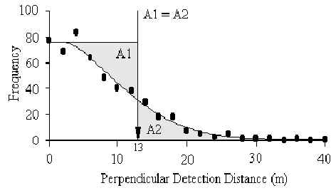 Figure 3.15.
Frequency distribution of perpendicular detection distances for the southern amazon red
squirrel (S. spadiceus). Program Distance computes the appropriate detection
function, and then calculates the distance where the area of A1 equals that of A2; in this
case 13 m.
Figure 3.15.
Frequency distribution of perpendicular detection distances for the southern amazon red
squirrel (S. spadiceus). Program Distance computes the appropriate detection
function, and then calculates the distance where the area of A1 equals that of A2; in this
case 13 m.
Table 3.12. Perpendicular detection distance (Psp), 95% CI, and appropriate distance decay model for 12 species for which sufficient data was collected. Distance decay models: HNC = Half-Normal/Cosine; UC = Uniform/Cosine; HC = Hazard/Cosine.
| Species | Psp (m) |
95% CI |
Distance Model |
Species | Psp (m) |
95% CI |
Distance Model |
|
| T. tetradactyla | 22 |
12 – 38 |
UC |
N. nasua | 27 |
20 – 36 |
UC |
|
| S. fuscicollis | 32 |
28 – 35 |
HC |
T. tajacu | 15 |
13 – 18 |
UC |
|
| S. boliviensis | 50 |
40 –62 |
UC |
M. americana | 15 |
11 – 21 |
UC |
|
| C. brunneus | 26 |
18 – 39 |
HC |
S. ignitus | 10 |
9 – 12 |
UC |
|
| A. seniculus | 30 |
24 – 39 |
HNC |
S. spadiceus | 13 |
12 – 14 |
HNC |
|
| C. apella | 39 |
33 – 47 |
UC |
D. variegata | 13 |
11 – 15 |
HC |
Table 3.13. Perpendicular detection distance (Psp), for 14 species for which insufficient data was collected to determine 95% CI.
| Species | Psp (m) |
. | Species | Psp (m) |
| M. tridactyla | 15 |
. | E. barbara | 18 |
| B. variegata | 1 |
. | G. vitata | 10 |
| Dasypus sp. | 5 |
. | L. longicauda | 24 |
| Aotus sp. | 13 |
. | L. pardalis | 46 |
| C. albifrons | 77 |
. | T. terrestris | 50 |
| A. paniscus | 63 |
. | T. pecari | 50 |
| A. microtis | 18 |
. | M. pratti | 13 |
Table 3.14. Density estimates for 12 mammal species (individulas/km2).
| Species | CAPH |
. | EI |
. | ECO |
. | SACHA |
. | TRC |
. |
| . | T |
C |
T |
C |
T |
C |
T |
C |
T |
C |
| T. tetradactyla | 0.0 |
0.0 |
0.5 |
0.0 |
1.1 |
1.1 |
1.2 |
0.0 |
0.5 |
0.0 |
| S. fuscicollis | 29.1 |
15.2 |
10.5 |
7.4 |
15.2 |
10.8 |
4.5 |
5.6 |
3.0 |
6.9 |
| S. boliviensis | 2.1 |
12.6 |
0.0 |
4.3 |
14.8 |
6.7 |
16.5 |
19.3 |
36.6 |
9.8 |
| C. brunneus | 0.8 |
0.0 |
2.6 |
1.3 |
0.0 |
0.0 |
0.4 |
0.0 |
0.5 |
5.4 |
| A. seniculus | 0.4 |
0.0 |
5.6 |
0.0 |
1.7 |
4.3 |
0.6 |
0.2 |
5.0 |
1.5 |
| C. apella | 0.0 |
1.4 |
4.8 |
12.0 |
3.9 |
4.9 |
0.3 |
1.8 |
11.9 |
9.5 |
| N. nasua | 0.2 |
0.0 |
0.0 |
0.2 |
1.7 |
2.5 |
0.0 |
4.1 |
2.5 |
0.0 |
| T. tajacu | 1.1 |
2.6 |
5.2 |
4.5 |
0.0 |
2.5 |
2.0 |
4.7 |
2.6 |
0.7 |
| M. americana | 0.0 |
0.6 |
0.0 |
1.2 |
0.0 |
1.1 |
0.4 |
1.1 |
0.3 |
0.4 |
| S. ignitus | 4.8 |
5.8 |
3.8 |
1.9 |
1.4 |
0.7 |
4.7 |
3.4 |
8.9 |
5.1 |
| S. spadiceus | 31.9 |
24.7 |
18.4 |
9.5 |
23.0 |
16.9 |
10.8 |
13.7 |
8.9 |
16.2 |
| D. variegata | 11.8 |
5.4 |
4.0 |
6.0 |
1.7 |
5.5 |
7.6 |
7.7 |
1.8 |
1.5 |
Forage Scrapings
A total of 342 individual quadrat searches were made over the period of the study, for an average of 3.1 searches per quadrat and a total search area of 13.7 hectares (Table 3.15). This search effort encountered a total of 751 forage scrapings, the overall distribution of which was found to be significantly clumped and characterised by a negative binomial distribution (Figure 3.16), as shown by the values of Index of Dispersion (Observed variance/Observed mean) which are generally larger than 1. A paired t-test revealed that the average density of scrapes along T transects was found to be significantly lower than along C transects (t = -3.37, p < 0.03), a trend that is evident from figure 3.17. Furthermore, a Pearson correlation coefficient revealed a significant negative correlation between traffic and scrape density near T (Pearson = –0.92, p < 0.05).
Table 3.15. Summary of scrapings data. Each quadrat = 0.04 ha.
| Lodge | . | No. of quadrats sited |
No. of quadrats searched |
Equiv. area searched (ha) |
No. scrapes found |
Ave. Density (scr/quad) |
VAR |
Index of Dispersal |
| CAPH | T |
16 |
49 |
1.96 |
43 |
0.88 |
1.77 |
2.02 |
| . | C |
13 |
35 |
1.40 |
73 |
2.09 |
4.54 |
2.18 |
| EI | T |
7 |
23 |
0.92 |
24 |
1.04 |
2.50 |
2.40 |
| . | C |
7 |
24 |
0.96 |
156 |
6.50 |
40.58 |
6.24 |
| ECO | T |
11 |
40 |
1.60 |
36 |
0.90 |
2.86 |
3.18 |
| . | C |
13 |
52 |
2.08 |
119 |
2.29 |
3.03 |
1.32 |
| SACHA | T |
9 |
26 |
1.04 |
36 |
1.38 |
4.67 |
3.37 |
| . | C |
9 |
24 |
0.96 |
146 |
6.08 |
19.54 |
3.21 |
| TRC | T |
13 |
35 |
1.40 |
50 |
1.43 |
1.54 |
1.08 |
| . | C |
12 |
34 |
1.36 |
68 |
2.00 |
1.82 |
0.91 |
| Total | . | 110 |
342 |
13.68 |
751 |
2.20 |
9.73 |
2.59 |
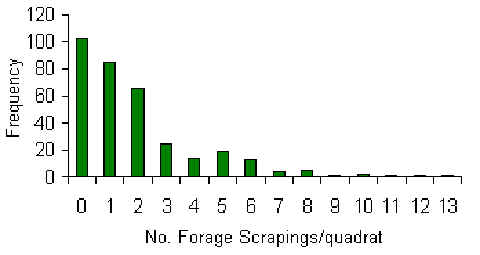
Figure 3.16. Frequency distribution of number of forage scrapings per quadrat.
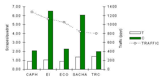
Figure 3.17. Scrape density along T and C at each lodge.