In his Organon, Aristotle called this particular process of reasoning epagwgh (epagoge), since then, disregarding its most rudimentary formulations, speculations on this has lain dormant for several centuries until its serious reconsideration was ignited by the scientific revolution. In the preceding chapter we have defined inductive argument as "an argument whose premises are meant to support the conclusion only with probability, and this probability is dependent upon what else may be the case." In this chapter, we are going to study in closer detail this argument.

Consider yourself a freshman in college who in your first semester happened to enroll in the mathematics class of Prof. Rivera. You found his class lively and challenging. The succeeding semester, you were again in the higher mathematics class of Prof. Rivera, and again you found it lively and challenging. By this time an idea is gradually forming in your head that probably all the mathematics classes of Prof. Rivera are lively and challenging, and given another opportunity, you will gladly be in his class again for the succeeding terms. For that particular matter, you are reasoning inductively using your past experiences as the premises. This is in fact the very foundational idea of upon which induction rests: learning from experience.

Through experience, we can spot several instances of patterns, regularities, resemblance and similarities. These may occur in simple and everyday moments, such as knowledge that traffic is garbled in Metro Manila in between 7:00 to 9:00 A.M. on weekdays, or in complicated and scientific settings that water when subjected to hydrolysis would decompose into oxygen and hydrogen. A correct induction is merely the extension of the patterns, regularities, resemblance and similarities that we already learned from experience to the future and unknown experiences. For instance, based on our past knowledge that traffic has always been garble in Metro Manila in between 7:00 to 9:00 A.M. on weekdays, we draw the conclusion that on the next weekday, and all weekdays hereafter, traffic will always be garbled in Metro Manila in between 7:00 to 9:00 A.M. Induction is a matter of using the known past as the basis for predicting the unknown future.

Comparing the inductive and the deductive arguments, we will notice at least two salient differences. First, as mentioned in the preceding chapter, the conclusion of correctly constructed inductive argument is always less certain than its premises; whereas the conclusion of a correctly constructed deductive argument is as certain as its premises. Hence, the conclusion of the inductive argument.

All Philippine wild cats encountered so far by man are unfriendly. So, probably all Philippine wildcats are unfriendly.

is not as certain as the conclusion of the deductive argument

All mammals are vertebrates. Philippine wildcats are mammals. So, Philippine wildcats are vertebrates.

"So, Philippine wildcats are vertebrates" is certain and absolute, while "So, probably all Philippine wildcats are unfriendly" is only probable and can be provisionally accepted as true until a contrary instance is brought about. It is this uncertainty, this provisional nature of the inductive conclusion that bothered the early modern theorists of inductive logic.

But the second major difference between these two types of argument redeems the previously mentioned shortcoming of inductive reasoning. Unlike the deductive conclusion, the conclusion of a correctly constructed inductive argument is neither pre-contained nor implied in and by its premises. For instance in the same inductive argument, the conclusion "Probably all Philippine wildcats are unfriendly" is neither pre-contained, nor implied in and by the premise "All Philippine wildcats encountered so far by man are unfriendly"; while in the case of the deductive argument mentioned above, the conclusion "Philippine wildcats are vertebrates" is already implied by the two premises. In simpler words, inductive arguments give us new information, whereas deductive arguments simply rearrange the given information in the premises to make explicit what was previously implied. Hence, deductive argument has been called transmitter of truth and preserver of truth, while inductive argument has been called discoverer of truth.

The fact that the inductive argument gives new information points out its great value as a method of acquiring knowledge. Yet, this great value of inductive argument is acquired at the expense of certainty. Unlike valid deductive arguments, even the best inductive argument involves the element of risk. No matter how true the premises of an inductive argument may be, no matter how perfect its inference may be. Its conclusion is not guaranteed to be 100% true and certain. Every time we reason inductively, we always perform the inductive leap from the premises to the conclusion, and through this inductive leap we may find ourselves standing on new terrain of knowledge or falling into the abyss of errors. Induction is wresting new knowledge from the clutches of uncertainty.

INDUCTION AND UNCERTAINTY

Once we admit the uncertainty of the outcome of the inductive leap, we admit at the same time that its outcome can either be true or false. The next question that would come to our minds would be on percentage: how certain?, or how uncertain would our conclusion be?. This question naturally leads us to the idea of calculating probabilities.

THE PROBABILITY CALCULUS

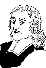Blaise Pascal (1623-1662): French philosopher, theologian, mathematician and physicist, who is considered as one of the founders of the mathematical theory of probability.

What is today considered an impressive branch of mathematics, had a rather sinister origin. Blaise Pascal, though himself a respected scholar and an inspiring philosopher and theologian, owing to a poor health, had to heed medical advice and find diversion in Paris by leading a frivolous life for a while. Among the frivolities of this sojourn was the games of chancein the Parisian gambling dens. It was at this point in Pascal's life when his scholarly and inquisitive mind encountered the too mundane questions regarding the odds of winning against that of loosing in various games of chance. This marked the beginning of the serious study of probability. Later on, Pascal collaborated with the lawyer and mathematical buff, Peirre de Fermat. If at this point we find gambling indeed too sinister to engender probability calculus, well, everything was in fact not that sinister for the ancestry of probability calculus includes the sordid and the macabre. Probability calculus had another impetus from the ghastly research of the English haberdasher, turned public servant, turned military man, John Graunt (1620-1674), who rummaged through the death records of the London parishes kept since 1532 and published the Observations upon the Bills of Mortality, which is today considered seminal not only for probability calculus but for statistics as well and earned him the title father of demography. Today, probability calculus has applications to insurance policy making, quality control in manufacturing, studies of heredity and population growth, weather forecast, and quantum physics.

The Basic Formula for Probability

 

Probability calculus is an a priori discipline. That means its body of knowledge is not something gleaned from experimentation or observation of objects from the real world, but through mental investigations and mathematical deductions. In this calculus, the probable is scored from 0 to 1. 0 for the absolutely improbable, 1 for the highly probable or certain, and the varying fractions in between 0 and 1 for the different degrees of certainty. The basic formula for figuring out specific scores is

P(A) = n/S

Where P (A) stands for probability of event A; n for event A's number of outcomes, or simply the number of favorable outcome; and S for sample space, or the number of all possible outcomes. A coin, for instance, has two sides and therefore has a sample space of 2 outcomes. Hence if one tosses a coin and bet for a head, the probability of predicting it right is

P(A) = n/S P(A) = head / head and tail P(A) = 1/2

And if one throws and die and bet for a six to roll out, the probability of predicting it right is

P(A) = n/S P(A) = six/ one, two, three, four, five and six P(A) = 1/6

The rule is, the bigger the fraction, the higher the probability. Thus, predicting that a head will come out from a toss of a coin is more probable than predicting that a six will roll out from a throw of a single die.

For roulette, an 18^th century game which has now become a fixture to almost any casino in the world, its wheel has slots which are non-consecutively numbered 1 to 36 with the addition of 0 and 00. That makes the size of its sample space 38. Winning is a matter of guessing the number of the slot on which the spinning ball would rest. There are several modes of betting, among which are one-number bet, two-number bet, three-number bet, four-number bet and six-number bet. The n varies in accordance to the mode of betting. Probability for one-number bet is

P(A) = n/S P(A) = 1/38

It follows that for two-number bet, probability is 2/38, or 1/19; for three-number bet, 3/38; for four-number bet, 4/38, or 2/19; and for six-number bet 6/38, or 3/19.

The basic formula applies only to the computation of probabilities of single events. In figuring out the probabilities of combined events the basic formula will be modified accordingly.

On Joint Probabilities

 

P(A & B) = P(A) x P(B)

The simplest application of this derivative formula is the calculation of the joint probability of events that are independent from each other. By independent events we mean events in which the result of one would not affect the result of the other and vice versa. For instance, if we toss two coins, the outcome of one coin would in no way affect the outcome of the other. Hence, if we bet that two heads would come out after a toss of two coins, the probability would be

P(A & B) = P(A) x P(B) P(A & B) = (n/S) x (n/S) P(A & B) = (1/2) x (1/2) P(A & B) = 1/4

If we bet that after a throw of two dice two sixes will roll out, our probability of predicting it right would be

P(A & B) = P(A) x P(B) P(A & B) = (n/S) x (n/S) P(A & B) = (1/6) x (1/6) P(A & B) = 1/36

Within Manila and some other points in the country there is a very popular game of chance based on the scores of the competing teams in the Philippine Basketball Association (PBA). We call this ending, and its rules are quite simple. The one who predicts the last digits of the scores of each team wins. The score of the winning team represents the first digit of the winning combination and the score of the losing team, the second. Hence, if the PBA teams ended up with the score 80-76, the winning ending combination is 0-6. Notice that whatever the score of the first team would in no way affect that of the second, thus they are independent events and the product theorem can be applied immediately. Since for either digit of the winning combination there are 10 possible outcomes (0, 1, 2, 3, 4, 5, 6, 7, 8 or 9), each digit has sample space size of 10. The probability of guessing the winning combination would then be

P(A & B) = P(A) x P(B) P(A & B) = (n/S) x (n/S) P(A & B) = (1/10) x (1/10) P(A & B) = 1/100

and that is a rather slim chance of guessing it right.

There are instances however, when the result of the first event can affect the other event. For instance, the chance of getting a black ace and a black jack after two picks from a deck of 52 cards, n and S vary in the first and second pick. For the first pick, n is 4 (that is either one of A�, A�, J� or J�) and S is 52. For the second pick, n would be reduced to 2 (If a black ace has been taken during the first picking, we are left with J� or J� or if a black jack has been taken, we are left with A� or A� and S would be reduced to 51. Thus the probability would be

P(A & B) = P(A) x P(B) P(A & B) = (n/S) x (n/S) P(A & B) = (4/52) x (2/51) P(A & B) = 8/2,652 P(A & B) = 2/663

The same principle can applied in computing the chances of winning the jackpot price in our government sponsored Lotto. In this game an urn mechanically spins and expels out six balls from a collection of forty-two numbered from 1 to 42. Guessing the six numbers means jackpot. Since we bet on six numbers and the urn expels out the balls one at a time, n and S decrease every after expulsion. Hence, the probability of guessing the six numbers would be

P(A, B, C, D, E & F) = P(A) x P(B) x P(C) x P(D) P(E) x P(F) P(A, B, C, D, E & F) = 6/42 x 5/41 x 4/40 x 3/39 x 2/38 x 1/37 P(A, B, C, D, E & F) = 720 / 3,776,965,920 P(A, B, C, D, E & F) = 1 / 5,245,786

Quite a miscroscopically slim chance of hitting the jackpot!

On Fair Gambling

 

Bet : Payoff = n : (S-n)

Hence, if one bets for the head in an honest toss of a single coin, the fair ratio would be

Bet : Payoff = n : (S-n) Bet : Payoff = 1 : (2-1) Bet : Payoff = 1 : 1

That means, if one bets P10 the payoff should be P 10. If one bets that a single dice will roll out six, the ratio should be

Bet : Payoff = n : (S-n) Bet : Payoff = 1 : (6-1) Bet : Payoff = 1 : 5

That means, if one bets P10 the payoff should be P 50. Yet in many forms of gambling, most specially formal gambling, the actual ratio between bet and payoff is not fair. Take the roulette for example. For one-number bet, the fair ratio is

Bet : Payoff = n : (S-n) Bet : Payoff = 1 : (38-1) Bet : Payoff = 1 : 37

That means a P 10 bet should have a payoff of P 370. But casinos simply disregards the fair ratio and follows their own ratio of 1: 35 which shortchanges their patrons by 2 units. This very slight shortchanging, unnoticed by many gamblers, gives the casinos a big killing. It has been noted that roulette has an average yield that is 5.26% higher than the other casino games.

For ending, the fair ratio should be

Bet : Payoff = n : (S-n) Bet : Payoff = 1 : (100-1) Bet : Payoff = 1 : 99

But again, this fair ratio is disregarded, in favor of an unfair ratio of 1:80.

For Lotto, fair ratio should be

Bet : Payoff = n : (S-n) Bet : Payoff = 1 : (5,245,786 - 1) Bet : Payoff = 1 : 5,245,785

Thus, ideally a P10 bet should win P52,457,850, but again that prize is not immediately posted.

The above mentioned examples clearly demonstrates the hidden unfairness included in many games of chance. For sure, these games entertain us well. They can be a good diversion from the working man's daily tensions and pressures, in fact Pascal himself used them that way to improve his health. But once we think of them as a way of getting richer that is when the evils of gambling start. If the actual ratio between bet and payoff is lower than that of the fair ratio, gamblers would always be losers in the long run, for their efforts would amount to taking a chance against chance itself, or hoping against hope itself.

SOME GUIDELINES FOR HIGHER PROBABILITIES

Probability calculus is indeed very effective in figuring the level of certainties of many events. Coupled with statistics, it can very well determine the probability of any given inductive argument. For example, probability calculus and statistics can easily determine the certainly of the conclusion for the argument

Tomas Cruz is a Filipino and is hospitable. Andres Reyes is a Filipino and is hospitable. Reynaldo de Jesus is a Filipino and is hospitable. Quintin Rivera is a Filipino and is hospitable. Therefore, probably all Filipinos are hospitable.

Aside from figuring out mathematically the levels of certainty, logic offers a set of more handy principles for ensuring higher probability in inductive reasoning.

FORMS OF INDUCTIVE ARGUMENTS

In the preceding chapter, in our discussion on validity and invalidity, we mentioned that such qualities are applicable only to deductive arguments and that inductive arguments are evaluated only as better or worse. The reason for such a distinction is the fact that inductive arguments are content-dependent, while deductive arguments are form-dependent. This means we cannot appreciate induction apart from its contents, just as we cannot appreciate deduction apart from its formula. Hence, forms are not as vital to inductive arguments as they are to deductive arguments. However, it is only through the study of forms of induction that we can have chances of attaining the better induction most of the time and avoiding the worse ones. For this section, we are going to go through six different inductive forms, with the sixth form having five sub-forms.

ENUMERATIVE INDUCTION

The most common form of induction is the one that comes immediately to our mind when we hear the word inductive argument, the enumerative induction.

a is P and has the attribute x. b is P and has the attribute x. c is P and has the attribute x. So, probably all P's have the attribute x.

This form moves from the fact that two or more things belong to the same category P and have the same attribute x, to the conclusion that all things that belong to category P have the attribute x. The following arguments are examples of this form.

Rizal is a hero and was full of courage. Aguinaldo is a hero and was full of courage. Bonifacio is a hero and was full of courage. Therefore, probably all heroes were full of courage. Van Gogh is a famous painter who ground his own pigments. Renoir is a famous painter who ground his own pigments. Dali is a famous painter who ground his own pigments. So, probably all famous painters ground their own pigments.

Francis Bacon (1561-1626): British politician, essayist and philosopher of science who re-awakened the speculations on induction.

There are actually two types of enumerative induction, the perfect and imperfect. Perfect enumerative induction covers the whole sample space with its premises, and the imperfect covers only part of the sample space. More often than not, when we use this inductive form, we are in fact using its imperfect type. Since, structurally speaking the premises, each covering the individual instances, are always limited in number, enumerative induction is prone to disregard the principles for higher probability. To this the British philosopher Sir Francis Bacon (1561-1626) sardonically remarked: "For the induction which proceeds by simple enumeration is childish; its conclusions are precarious and exposed to peril from a contradictory instance: and it generally decides on too small a number of facts, and on these only which are at hand." Actually, Bacon was the one who re-awakened the speculations on inductive logic which for the past many centuries had lain dormant. He entitled his major work Novum Organum (New Organon), a provocative allusion to Aristotle's Organon whose tenets he wanted to raze with a new inductive logic.

ANALOGICAL INDUCTION

Another form of induction, which is actually derived from ordinary day reasoning is the analogical induction.

a, b, c, d all have the attribute P and Q. a, b, c have the attribute R. So, probably d also has the attribute R.

This form of inductive argument moves from the fact that two or more things are similar in one or more aspects P and Q to the conclusion that they are similar in some further aspect R. The following are its examples.

Doves, sparrows, parrots and cassowaries are all birds. Doves, sparrows, and parrots are oviparous. So, probably cassowaries are also oviparous. Physics, chemistry, biology and neurology are natural sciences. Physics, chemistry and biology are based on empirical facts. So, probably neurology is also based on empirical facts.

STATISTICAL SYLLOGISM

With its syllogistic form,

n% of P has the attribute x. a is a member of P. So, probably a has/does not have the attribute x.

the statistical syllogism may appear like a categorical deductive syllogism. Yet it varies distinctly from the latter in the sense that its outcome remains in the parameters of inductive uncertainty. It moves from some portion n% of a given category P to one particular member a of category P as having or not having the attribute x.

Only 10% of the Filipinos are rich. Pedro Javier is a Filipino. Thus, probably Pedro Javier is not rich. Most Filipino executives in Indonesia are highly respected. Mr. Andres San Sebastian is a Filipino executive in Jakarta. So, probably he is highly respected.

The particular member's having or not having the attribute x is decided by the actual value of n%. Values higher than 50% means the particular member has the attribute x, and values lower than 50% means the contrary. Though values equivalent to either 0% or 100% will not make a statistical syllogism, for that would amount to a deductive categorical syllogism, values nearer to 0% and 100% make higher probabilities compared to values nearer to 50%. Often, percentages is substituted with non-numerical quantifiers such as most, few, generally, rarely, and the like.

INDUCTIVE GENERALIZATION

A stronger version of the enumerative induction is the inductive generalization.

n% of observed P has the attribute x So, probably n% of all P's have the attribute x.

This inductive form moves from an observed portion of a given category P to the whole of P. Statistical surveys and researches employ this inductive form.

All (100%) wildcats encountered men are ferocious and unfriendly. So, probably all wildcats are ferocious and unfriendly. 60% of the HIV patients at the Philippine General Hospital are gay. So, probably 60% of all HIV patients are gay.

If enumerative induction cites instances one at a time in its premises, inductive generalization cites them collectively in its single premise. Structurally speaking, the premise of the latter has a wider scope compared to those of the former. Hence, potentially the latter has a higher claim to probability.

ABDUCTIVE INDUCTION

The structure of abductive induction

There is q If p then q So, probably p.

strikingly resembles that of a particular form of deductive argument called modus ponens which has the structure of.

If p then q there is p So, there is q.

As a deductive argument, given true premises, modus ponens produces absolutely certain conclusions. Thus, the conclusion in the argument

If you drink alcohol excessively, then you ruin your liver. You are drinking alcohol excessively. Therefore, you are ruining your liver.

flows necessarily and absolutely from the premises. While the conclusion of the abductive induction

There are strong winds. If the storm breaks, then there will be strong winds. So, probably the storm has broken.

is only probable. Abductive induction moves from the consequent q, followed by the hypothetical claim if p then q which serves as the background theory, and finally towards the probable conclusion that q is caused by the antecedent p.

Though abductive induction is deductively invalid, it has practical values as an inductive argument. For instance, we have it as a background theory that if there is a power blackout, then there will be no electricity in one's home. The fact that there is a blackout necessarily implies that there will be no electricity in one's home. This is how the deductive modus ponens proceeds. But reversing the situation would not result to certainty. The fact that there is no electricity in one's home does not necessarily imply that there is a power blackout, for such a case of not having electricity in one's home can be caused by some other factors other than a power blackout. Abductive induction counts on the probability that the fact that there is no electricity in one's home is caused by a power blackout. The ch can be used as a starting point for further verification. The process of medical diagnosis and the construction of scientific hypotheses actually employ this inductive pattern.

Abductive induction, if viewed from the perspective of the deductive modus ponens would certainly appear anomalous and invalid. But if used properly as an inductive argument it has its own values and merits.

CAUSAL REASONING: MILL'S METHOD

Aristotle was not only a logician and philosopher, he was also a biologist and scientist. In fact, he was the first one to establish a scientific school in western history. In Aristotle's system of scientific investigation , there are four types of causes: the material, the formal, the efficient and the final. Material cause refers to that element/s which a thing under investigation is constituted, or simply the material/s which the thing is made of. Formal cause refers to the patterns and specifications in the maker's mind which gave the thing its present nature and characteristics. The efficient cause refers to the labor involved in the production of the thing. And the final cause refers to the goal for which the thing is produced. In the Aristotelian system what is given more emphasis is the search for final cause. Hence, we have the teleological model of investigation that explains things in view of its purpose. However, Francis Bacon pointed out this fundamental shortcoming of Aristotelian science and insisted that the search for the final cause and even for the formal cause are good only for metaphysical speculations, science should deal only with material and efficient causes. Hence, in modern scientific investigations the old Aristotelian teleological model has been supplanted with the Baconian causal model that will explain things in terms of their material and efficient causes alone.

For modern science knowledge of things to a large extent means knowledge of their causes, causes in its Baconian sense. Hence, once cause and effect are properly identified

or once the cause of a given effect is identified, or once the effect of a given cause is identified, scientific knowledge is attained. But the neat coupling of cause and effect represented in the diagram above, more often than not happens only in the controlled parameters of the laboratory. In the real world what we find mostly are

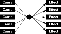
complex networks of causes and effects. Even if Bacon successfully streamlined the idea of cause by excluding the final and formal causes, the modern science's search for the specific pair of cause and effect remains complicated.

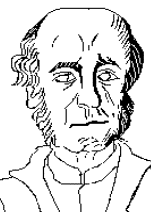John Stuart Mill (1806-1873): British philosopher, social and political thinker, who continued Bacon's cause against Aristotelian deduction and formulated five patterns of causal arguments.

The British philosopher, social and political thinker, and major proponent of the utilitarian school of thought, John Stuart Mill (1806-1873), continued Bacon's struggle against the Aristotelian deductive system and formulated five patterns of causal reasoning: the method of agreement, the method of difference, the joint method of agreement and difference, the method of residue, and the method of concomitant variation.

Causal reasoning is an inductive tool capable of establishing the link between specific causes and effects from the complex network of causation that we find in the real world. This may involve the identification of the specific cause, or effect, or the indispensable part of the cause. Echoing the Scottish David Hume's (1711-1776) famous necessary connexion, Mill defines cause as an "immediate, unconditional and invariable antecedent." Mill's contribution to is helpful as research tool for both the natural and the human sciences.

The Method of Agreement

 

A B C D occur together with w x y z B E F G occur together with w t u v So, probably B is the cause of w.

Think for example, this scenario of petty theft cases in the office of Prof. De Jesus. On the first day of the week, the professor lost his silver pen, and he can recall quite well that the only persons who entered his office were John, Mark, Gary and Ray. On the second day of the same week, he lost his antique letter opener, and he can also recall that the only persons who entered his office that day were John, Ray, and Patrick. On the third day, the professor lost a volume of his leather bound Greek Drama, and he can also recall that only Paul, Ray, Mark and Greg visited his office that day. On the fourth day, the professor lost his gold-rimmed spectacles, and only Gary, John, Mark and Ray visited him that day. Among the persons who entered the office of Prof. De Jesus, who could possibly be the mischievous crook? By using Mill's method of agreement we can assemble our clues as

(1st day):	John, Mark, Gary &Ray		Theft (silver pen)
(2nd day):	John, Ray, & Patrick		Theft (antique letter opener)
(3rd day):	Paul, Ray, Mark & Greg		Theft (leather bound volume)
(4th day):	Gary, John, Mark & Ray		Theft (gold-rimmed spectacles)
	So, probably Ray		Theft

Since Ray is the common circumstance, or he has been consistently present in the crime scene from day 1 to day 4, we are justified in concluding that probably he is the one responsible of the mysterious disappearance of Prof. De Jesus' precious articles. That is just a scenario of how the method of difference can be useful. Let us take a look how this method can be used in the social sciences. Sociologists knew before that urban death rate is higher compared to the rural. But they were uncertain regarding its cause, is it urbanization as such or industrialization. In the late 60's this question was settled by comparative study on three groups of urban centers. The first group of cities are commercial urban centers (urbanization and commerce), the second group are industrial urban centers (urbanization and industrialization), and the third group are urban centers that are seats of central government (urbanization and government). The sociologist found out that throughout the three groups death rate is consistently high,

(1st group):	urbanization & commerce		High death rate
(2nd group):	urbanization & industrialization		High death rate
(3rd group):	urbanization & government		High death rate
	So, probably urbanization		High death rate

Hence, they have enough reason to conclude that it is urbanization and not industrialization that causes the strikingly higher urban death rate.

The Method of Difference

 

A B C D occur together with w x y z A C D occur together with x y z So, probably B is the cause of w.

On May 14, 1876, Louis Pasteur (1822-1895), a French chemist and today honored as and founder of microbiology, made an investigation that put to rest the old belief in spontaneous generation. For his first set up, he poured some kind of broth into a flask and left it open to air contact for several days. For the second, he poured an equal amount of the same broth into another flask, sealed it tightly from air contact and left it for an equal number of days. After the equal period lapsed, microorganisms developed in the open flask which were absent in the sealed flask.

(1st set-up):	broth, flask, air contact, n days		micro-organisms
(2nd set-up):	broth, flask, n days
	So, probably air contact		micro-organisms

Knowing that the only difference between the two set-ups is the contact/non-contact with air, Pasteur concluded that contact with air caused microorganisms to develop in the open flask. Hence, he demonstrated that the organisms that developed in the broth were not generated spontaneously, but were airborne. This experiment led to the development of the famous process of pasteurization.

The Joint Method of Agreement and Difference

 

ABCD occur together with wxyz		ABCD occur together with wxyz
BEFG occur together with wtuv		ACD occur together with xyz
So, probably B is the cause of w.

This method can be best illustrated with a reconstruction the experimental set-up used by the Dutch physician and Nobel prize winner Christiaan Eijkman (1858-1930) in his investigations on the proper functioning of the nervous system and carbohydrate metabolism. Our reconstruction will show two groups of set-up, each having two set-ups. In the first group, for the first set-up, we have five fowls fed with polished rice and unsterilized water. For the second set-up of the same group, we have five fowls fed with polished rice and sterilized water. In the second group, for the first set-up, we have five fowls fed with unpolished rice and sterilized water. For the second set-up of the second group, we have five fowls fed with fed with polished rice and sterilized water. All the fowls from the two set-ups of the first group developed a deficiency disease called beriberi. Only the fowls from the second set-up of the second group developed the same deficiency disease.

	First Group					Second Group
(1st set-up)	PRice & UWater		Beriberi		(1st set-up)	URice & SWater
(2nd set-up)	PRice & SWater		Beriberi		(2nd set-up)	PRice & SWater		Beriberi
	So, probably Polished Rice				Beriberi

Using the method of agreement for the first group we can infer that the diet of polished rice is causally related to the development of beriberi in both set-ups. Using the method of difference for the second group we can infer that again the diet of polished rice is causally related to the development of beriberi in the second set-up. Through the joint method of agreement and difference, we can know with a higher probability that the diet of polished rice is causally related to the development of beriberi. Of course, Dr. Eijkman knew that the reason why the diet of polished rice is deficient is due to the fact that in polishing away the bran from the rice a rich supply of vitamin B1 (thiamine) is lost.

The Method of Residue

 

A B C occur together with w x y B is previously known to be the cause of w C is previously known to be the cause of x So, probably A is the cause of y.

Imagine for example a certain pastry that you bought from a specialty shop. Upon tasting it you loved its sweet, crumbly, chocolate taste and its pungent nutty flavor. You were curios about that pungent nutty flavor. The package says the pastry is made of flour, butter, cocoa powder, sugar and marsala. Knowing that the pastry's sweetness is due to sugar, it crumbly characteristic is due to flour and butter, and its chocolate taste is due to cocoa butter, then you are justified in saying that it is marsala that causes its pungent nutty flavor.

Flour, butter, cocoa powder, marsala		sweet, crumbly, chocolate, pungent nutty flavor
Flour, butter		crumbly
Cocoa powder		chocolate
So, probably marsala		pungent nutty flavor

The same method was used by the Renaissance scientists who tried to settle the old question whether air has weight of not. The issue may appear a little silly for us, but at that time they were really serious about this debate. Some ancient and medieval scientists thought before that air is weightless, and some even went further that air has negative weight. Through an experiment with balloons, the issue was finally laid to rest. An uninflated balloon was weighed. Say, its weight was 10 ounces. It was inflated and weighed again. Say, the weight now is 13 ounces.

(Inflated Ballon):	uninflated balloon & air		10 ounces & 3 ounces
(Uninflated Balloon):	uninflated balloon		10 ounces
	So, probably air		3 ounces

Since there is an otherwise unexplainable increase of weight, the Renaissance scientists concluded that air indeed has weight.

The Method of Concomitant Variation

 

A B C occurs together with x y z A - B C occurs together with x - y z A+ B C occurs together with x+ y z Therefore, probably A is causally connected with x.

For example, sociologists and economists have noted the relationship between economic status and energy consumption. As of the last decade, countries with very high income have energy consumption of 4,257 kg. of coal equivalent per capita; countries with high income have energy of consumption of 2,913; countries with medium income have energy consumption of 414; and countries with low income have energy consumption of 62.

Countries with very high income		4,257 kg. per capita
Countries with high income		2,913 kg. per capita
Countries with medium income		414 kg. per capita
Countries with low income		62 kg. per capita
So, probably a country's income		per capita consumption of energy

Hence using the method of concomitant variation, and noting beforehand that energy consumption directly varies with economic status, these sociologists and economists have enough reason to conclude that economic status is casually related to the per capita consumption of energy. Today, this finding is taken for granted and energy consumption has been used as an indicator of progress.

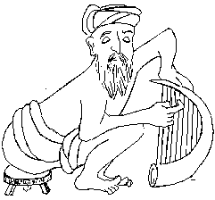For the method of concomitant variation, the relation of variation can be directly proportional as in the case mentioned above where energy consumption rises with economic status, or it can be inversely proportional like the following case. As early as the 6th century B.C., the Greek mathematician, astronomer and philosopher, Pythagoras of Samos (c560-c480 B.C.), had already employed this type of reasoning in his mathematical speculations on the theory of music. He noticed that with stringed instruments pitch is inversely proportional to thelength of the string. If a string is shortened, the pitch increases, and when its lenght is increased, the pitchdecreases. Hence, Pythagoras infered that the length of musical strings is causally related to the pitch.

CHAPTER SUMMARY

As we close this second chapter, again it would be fitting to make some retrospect on the things in inductive logic that we have examined. First, we have learned that the induction is fundamentally based on learning from the past experiences and projecting them into the future. Second, we have seen advantages and disadvantages of induction in comparison with deduction. If the inductive argument only offers probability, deduction offers certainty. But induction is a discover of truth while deduction is only its transmitter and preserver. Third, we plunged ourselves into the mathematical world of probability calculus and then into the practical principles for higher inductive probability. Lastly, we went into some cursory studies on the different inductive formulas: namely, the enumerative induction, the analogical induction, the statistical syllogism, the inductive generalization, the abductive induction, and the five methods of Mill's causal reasoning.