Coherent p - pulses and chirped quasi-solitons in a Kerr-lens mode-locked laser with a semiconductor absorber

2000©Vladimir L. Kalashnikov

Abstract

Application Areas/Subjects: Science, Physics, Applied Examples, Differential Equations, Laser Physics, Nonlinear Optics

Keywords: Ultrashort pulse, solid-state laser, semiconductor absorber, Kerr-lens mode locking, Bloch equations, ultra-short pulse

As one can see from "Solitons and quasi-solitons in the lasers: basic conceptions'', there is a quasi-soliton generation in the Kerr-lens mode-locked laser with a coherent semiconductor absorber. A condition of the quasi-soliton generation in the presence of self-phase modulation and group-velocity dispersion is the pulse chirp compensation. In the other words, the coherent quasi-soliton in the absorber corresponds to the Schrödinger quasi-soliton of the laser part of a master equation. Note, that the quasi-soliton of the master equation containing the laser and absorber parts is the soliton-like solution of each part separately. This fact allows to find the solution-like solution as a common self-consistent solution of both parts of the master equation. Now, we will consider the possibilities of the chirped pulse generation. For this aim we have to modify the system of Bloch's equations:

> restart:
bloch_1:=diff(b(t),t)=q*rho(t)*w(t)-diff(phi(t),t)*a(t);
bloch_2:=diff(a(t),t)=diff(phi(t),t)*b(t);
bloch_3:=diff(w(t),t)=-q*rho(t)*b(t);

bloch_1 : = � �t  b(t) = q r(t) w(t) - ( � �t  f(t)) a(t)

bloch_2 : = � �t  a(t) = ( � �t  f(t)) b(t)

bloch_3 : = � �t  w(t) = - q r(t) b(t)

Here [(�)/(�t)] f(t) is the pulses' phase modulation (we will suppose that the shift of the pulse carrier frequency from the absorber resonance is equal to zero).

There is a soliton solution of this system [L. Allen and J. H. Eberly, Optical Resonance and Two-Level Atoms (Wiley, New York, 1975)]:

> sol_1 := b(t) = b0*sech(t/tp);
sol_2 := a(t) = a0*sech(t/tp);
sol_3 := w(t) = tanh(t/tp);
sol_4 := rho(t) = rho0*sech(t/tp);
sol_5 := diff(phi(t),t) = psi*tanh(t/tp)/tp;

sol_1 : = b(t) = b0 sech( t tp )

sol_2 : = a(t) = a0 sech( t tp )

sol_3 : = w(t) = tanh( t tp )

sol_4 : = r(t) = r0 sech( t tp )

sol_5 : = � �t  f(t) = y tanh( t tp ) tp

Here y is the pulse chirp. The substitution of the solution in the system produces:

> eq1 :=
expand(numer(simplify(subs(b(t)=rhs(sol_1),lhs(bloch_1)) - subs( {diff(phi(t),t)=rhs(sol_5),rho(t)=rhs(sol_4),
w(t)=rhs(sol_3),a(t)=rhs(sol_2)}, rhs(bloch_1))))/sinh(t/tp))=0;

eq2 := expand(numer(simplify(subs(a(t)=rhs(sol_2),lhs(bloch_2)) - subs({diff(phi(t),t)=rhs(sol_5),b(t)=rhs(sol_1)},
rhs(bloch_2))))/sinh(t/tp))=0;

eq3 := numer(simplify(subs(w(t)=rhs(sol_3),lhs(bloch_3)) - subs({b(t)=rhs(sol_1),rho(t)=rhs(sol_4)},rhs(bloch_3))))=0;

bloch_sol := allvalues(solve({eq1,eq2,eq3},{a0,b0,rho0})); #solutions for the pulses' and absorbers' parameters

 

eq1 : = - b0 - q r0 tp + y a0 = 0

eq2 : = - a0 - y b0 = 0

eq3 : = 1 + q r0 b0 tp = 0

bloch_sol : = {b0 = 1 � 1 + y2 ,  r0 = - � 1 + y2 q tp ,  a0 = - y � 1 + y2 }, {b0 = - 1 � 1 + y2 ,  r0 = � 1 + y2 q tp ,  a0 = y � 1 + y2 }

So, we have one physical solution r0 = [(�{1 + y²})/(q tp)],  b0 = - [1/(�{1 + y²})],  a0 = [(y )/(�{1 + y²})], and this solution exists both in the case of y = 0 (it is so-called p - soliton) and in the case of y0 (it is a chirped quasi-soliton with variable area). Note, that the p - soliton is unstable in the absorber due to noise amplification on the pulse tail because of lim _{t� �} w(t) = 1 (it corresponds to the full population inversion in the absorber). But the pulse chirp can transform the pulse stability conditions essentially (see L. Allen and J. H. Eberly, Optical Resonance and Two-Level Atoms (Wiley, New York, 1975)) and, additionally, the pulse stability can be changed in the presence of the lasing factors. In the last case, the soliton of the Bloch's system have to be the soliton-like solution of the laser part of a master equation:

> master_laser :=
alpha*rho(t)-gam*rho(t)+I*phi*rho(t)+diff(rho(t),`$`(t,2)) +I*disp*diff(rho(t),`$`(t,2))+ sigma/lambda²*Intensity(t)*rho(t)-
I*beta/lambda²*Intensity(t)*rho(t);

 

master_laser : = a r(t) - gam r(t) + I f r(t) + ( �2 �t2  r(t)) + I disp ( �2 �t2  r(t)) + s Intensity(t) r(t) l2 - I b Intensity(t) r(t) l2

> collect(expand(numer(simplify(subs( {Intensity(t)=rho0²*sech(t/tp)², rho(t)=rhs(sol_4)^(1-I*psi)}
,master_laser)))/(rho0*(rho0/cosh(t/tp))^(-I*psi))),cosh(t/tp)²);

eq4 := evalc(coeff(%,cosh(t/tp0)²));
eq5 := evalc(expand(%%-eq4*cosh(t/tp)²));

eq4 : = - y2 l2 + l2 + 2 disp l2 y+ a tp2 l2 - gam tp2 l2 + I (disp l2 - disp l2 y2 + f tp2 l2 - 2 y l2)

eq5 : = s r02 tp2 - 2 l2 + y2 l2 - 3 disp l2 y + I (3 y l2 + disp l2 y2 - b r02 tp2 - 2 disp l2)

Now we have to take into account the result of the solution of the Blochs' equations:

> eq6 :=
subs(rho0²=(1+psi²)/tp²,coeff(eq5,I));
eq7 := subs(rho0²=(1+psi²)/tp²,coeff(eq5,I,0));
eq8 := coeff(eq4,I);
eq9 := coeff(eq4,I,0);

 

eq6 : = 3 y l2 + disp l2 y2 - b (1 + y2) - 2 disp l2

eq7 : = s (1 + y2) - 2 l2 + y 2 l2 - 3 disp l2 y

eq8 : = disp l2 - disp l2 y2 + f tp2 l2 - 2 y l2

eq9 : = - y2 l2 + l2 + 2 disp l2 y+ a tp2 l2 - gam tp2 l2

In the beginning we will consider the bandwidth-limited pulses (i. e. the solitons with y=0).

> sys := {subs(psi=0,eq6)=0,
subs(psi=0,eq7)=0, subs(psi=0,eq8)=0, subs(psi=0,eq9)=0}:
solve(sys,{disp,sigma,phi,tp²});

{s = 2 l2,  disp = - 1 2 b l2 ,  f = - 1 2 b (a- gam) l2 ,  tp2 = - 1 a- gam }

The obtained result differs from one for the the 2 p- pulses (see "Solitons and quasi-solitons in the lasers: basic conceptions''): the Kerr-lensing parameter is greater in four times, the dispersion is less in four times because of p - pulses' amplitude is two times less than 2 p - pulses' amplitude. It should be noted, that the saturated gain is less than the linear loss. This fact causes the pulse stability against laser noise if the initial loss into absorber is less than the difference between linear loss and saturated gain.

Now we have to take into account the gain saturation obviously:

> Energy = 2*rho0²*tp:
eq10:=Pump*alphamx/(Pump+tau*Energy+1/Tr)-alpha:
eq11:=numer(simplify(subs({tp=1/sqrt(gam-alpha)},subs(rho0=1/tp, subs(Energy=2*rho0²*tp,eq10))))):
alpha_sol:=solve(eq11=0,alpha): #This is solution for the saturated gain

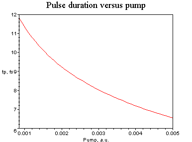
The dependence of the pulse duration versus dimensionless pump coefficient is:

> with(plots):
fig := plot( Re(evalf(subs(lambda=0.2,subs( {alphamx=0.1,Tr=300,tau=6.25e-4/lambda²,gam=0.01},
subs(alpha=alpha_sol[2],2.5/sqrt(gam-alpha)))))), Pump=0.00085..0.005,axes=boxed,labels=[`Pump, a.u.`, `tp,
fs`],title=`Pulse duration versus pump`,color=red):

display(fig,view=6..12);

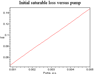
> plot( Re(evalf(subs(lambda=0.2,subs( {alphamx=0.1,Tr=300,tau=6.25e-4/lambda²,gam=0.01},
subs(alpha=alpha_sol[2],gam-alpha))))), Pump=0.00085..0.005,axes=boxed,labels=[`Pump, a.u.`,
`loss`],title=`Initial saturable loss versus pump`,color=red);

> sol_6 :=
subs(solve({eq8=0,eq9=0},{phi,tp²}),phi);
sol_7 := subs(solve({eq8=0,eq9=0},{phi,tp²}),tp²):
sol_8 := solve(eq6=0,disp):
chirp_1 := solve(numer(simplify(subs(disp=sol_8,eq7)))=0,psi)[3];
chirp_2 := solve(numer(simplify(subs(disp=sol_8,eq7)))=0,psi)[4];
disp_1 := simplify(subs(psi=chirp_1,sol_8));
disp_2 := simplify(subs(psi=chirp_2,sol_8));
sq_dur_1 := simplify(subs({psi=chirp_1,disp=disp_1},sol_7));
sq_dur_2 := simplify(subs({psi=chirp_2,disp=disp_2},sol_7));
inten_1 := simplify((1+chirp_1²)/sq_dur_1);
inten_2 := simplify((1+chirp_2²)/sq_dur_2);

sol_6 : = - - disp a+ disp gam + disp y2 a- disp y2 gam + 2 y a- 2 y gam - y2 + 1 + 2 disp y

chirp_1 : = 1 2 3 b+ � 9 b2 - 16 l4 - 8 l2 s+ 8 s2 l2 + s

chirp_2 : = 1 2 3 b- � 9 b2 - 16 l4 - 8 l2 s+ 8 s2 l2 + s

disp_1 : = - - 5 l4 b- 3 l2 b s- l 4 %1 - l2 %1 s+ 2 b s2 + 3 b3 + b2 %1 ( - 3 b2 - b %1 + 4 l4 + 4 l2 s) l2 %1 : = �   9 b2 - 16 l4 - 8 l2 s+ 8 s2

disp_2 : = - - 5 l4 b- 3 l2 b s+ l 4 %1 + l2 %1 s+ 2 b s2 + 3 b3 - b2 %1 ( - 3 b2 + b %1 + 4 l4 + 4 l2 s) l2 %1 : = �   9 b2 - 16 l4 - 8 l2 s+ 8 s2

sq_dur_1 : = - ( - 14 s3 b2 + 27 l2 s2 b2 - 12 l6 s2 + 5 l2 s2 b %1 - 4 l8 s+ 4 l4 s3 + 9 l2 b4 - 17 l6 b2 + 4 l10 + 4 l4 b %1 s+ 3 l2 b3 %1 + 24 l4 b2 s- 3 l6 b %1 - 18 b4 s- 2 s3 b %1 - 6 b3 %1 s+ 8 l2 s4) ( (l2 + s)2 ( - 3 b2 - b %1 + 4 l4 + 4 l2 s) l2 (a- gam)) %1 : = �   9 b2 - 16 l4 - 8 l2 s+ 8 s2

sq_dur_2 : = - ( - 3 l2 b3 %1 + 3 l6 b %1 - 4 l4 b %1 s- 5 l2 s2 b %1 - 14 s3 b2 + 27 l2 s2 b2 - 12 l6 s2 - 4 l8 s+ 4 l 4 s3 + 9 l2 b4 - 17 l6 b2 + 4 l10 + 24 l4 b2 s- 18 b4 s+ 2 s3 b %1 + 6 b3 %1 s+ 8 l2 s4) ( (l2 + s)2 ( - 3 b2 + b %1 + 4 l4 + 4 l2 s) l2 (a- gam)) %1 : = �   9 b2 - 16 l4 - 8 l2 s+ 8 s2

inten_1 : = - 3 2 ((a- gam) l2 ( - 3 b2 - b %1 + 4 l4 + 4 l2 s) ( - 2 l4 + 2 s2 + 3 b2 + b %1)) ( - 14 s3 b2 + 27 l2 s2 b2 - 12 l6 s2 + 5 l2 s2 b %1 - 4 l8 s+ 4 l4 s3 + 9 l2 b4 - 17 l6 b2 + 4 l10 + 4 l4 b %1 s+ 3 l2 b3 %1 + 24 l4 b2 s- 3 l6 b %1 - 18 b4 s- 2 s3 b %1 - 6 b3 %1 s+ 8 l2 s4) %1 : = �   9 b2 - 16 l4 - 8 l2 s+ 8 s2

inten_2 : = - 3 2 ((a- gam) l2 ( - 3 b2 + b %1 + 4 l4 + 4 l2 s) ( - 2 l4 + 2 s2 + 3 b2 - b %1)) ( - 3 l2 b3 %1 + 3 l6 b %1 - 4 l4 b %1 s- 5 l2 s2 b %1 - 14 s3 b2 + 27 l2 s2 b2 - 12 l6 s2 - 4 l8 s+ 4 l 4 s3 + 9 l2 b4 - 17 l6 b2 + 4 l10 + 24 l4 b2 s- 18 b4 s+ 2 s3 b %1 + 6 b3 %1 s+ 8 l2 s4) %1 : = �   9 b2 - 16 l4 - 8 l2 s+ 8 s2

Unlike "Solitons and quasi-solitons in the lasers: basic conceptions", there is the obvious condition for the value of l (in the absence of the chirp this condition is satisfied automatically):

> 9*beta²-8*lambda²*sigma+8*sigma²-16*lambda⁴ > 0;
solve(9*beta²-8*x*sigma+8*sigma²-16*x² = 0, x);

0 < 9 b2 - 16 l4 - 8 l2 s + 8 s2

- 1 4  s+ 3 4 �   s2 + b2   ,  - 1 4  s- 3 4 �   s2 + b2

That is l² - [(1 s)/4] + [(3 �{s² + b²})/4]. Additionally we have to find the solution for the saturated gain coefficient:

> Energy := 2*sqrt(gam-alpha)*A:
eq12 := Pump*alphamx/(Pump+tau*Energy+1/Tr)-alpha:
eq13 := solve(numer(simplify(eq12))=0,alpha):
sol_alpha_1 :=
subs(A=(1+chirp_1²)*sqrt(coeff(-1/sq_dur_1,(alpha-gam))),eq13[1]):
sol_alpha_2 :=
subs(A=(1+chirp_2²)*sqrt(coeff(-1/sq_dur_2,(alpha-gam))),eq13[1]):
sol_alpha_3 :=
subs(A=(1+chirp_1²)*sqrt(coeff(-1/sq_dur_1,(alpha-gam))),eq13[2]):
sol_alpha_4 :=
subs(A=(1+chirp_2²)*sqrt(coeff(-1/sq_dur_2,(alpha-gam))),eq13[2]):
sol_alpha_5 :=
subs(A=(1+chirp_1²)*sqrt(coeff(-1/sq_dur_1,(alpha-gam))),eq13[3]):
sol_alpha_6 :=
subs(A=(1+chirp_2²)*sqrt(coeff(-1/sq_dur_2,(alpha-gam))),eq13[3]):

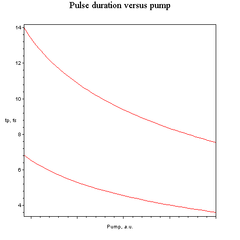
> fig2 :=
plot({Re(evalf(subs(lambda=0.2,subs( {beta=0.26,sigma=0.14,alphamx=0.1,Tr=300,
tau=6.25e-4/lambda²,gam=0.01 },subs(alpha=sol_alpha_4,2.5*sqrt(sq_dur_2)))))),
Re(evalf(subs(lambda=0.3,subs( {beta=0.26,sigma=0.14,alphamx=0.1,Tr=300,
tau=6.25e-4/lambda²,gam=0.01 },subs(alpha=sol_alpha_4,2.5*sqrt(sq_dur_2))))))},
Pump=0.00085..0.005,axes=boxed,labels=[`Pump, a.u.`, `tp, fs`],title=`Pulse duration versus pump`,color=red):

display(fig2);

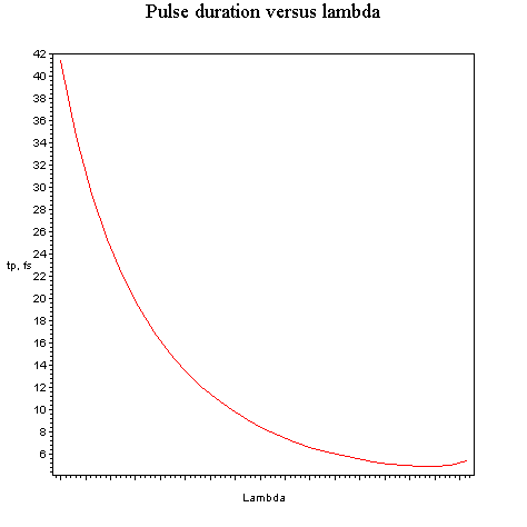
> lambda := 'lambda':
par1 := array(1..40):
par2 := array(1..40):
i := 1:
for lambda from 0.1 to 0.425 by 0.0125 do par1[i] :=
[lambda,Re(evalf(subs(Pump=0.001,subs( {beta=0.26,sigma=0.14,alphamx=0.1,Tr=300,
tau=6.25e-4/lambda²,gam=0.01 },subs(alpha=sol_alpha_4,2.5*sqrt(sq_dur_2))))))]:
par2[i] := [lambda,Re(evalf(subs({beta=0.26,sigma=0.14},chirp_2)))]:
i:=i+1: od:

plot([seq(par1[i], i=1 .. 27)],axes=boxed,labels=[`Lambda`, `tp, fs`],title=`Pulse duration versus lambda`);
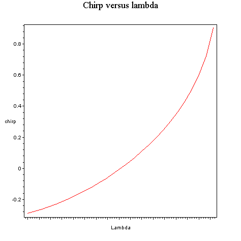
plot([seq(par2[i], i=1 .. 27)],axes=boxed,labels=[`Lambda`, `chirp`],title=`Chirp versus lambda`);

> lambda := 'lambda':
par2_2 := array(1..40):
i := 1:
for lambda from 0.1 to 0.425 by 0.0125 do par2_2[i] :=
[lambda,Re(evalf(subs({beta=0.26,sigma=0.14},sqrt(1+chirp_2²))))]:
i:=i+1: od:
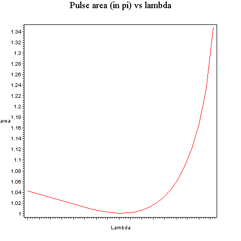
plot([seq(par2_2[i], i=1 .. 27)],axes=boxed,labels=[`Lambda`, `area`],title=`Pulse area (in pi) vs lambda`);

> lambda := 'lambda':
par3 := array(1..101):
par4 := array(1..101):
par5 := array(1..101):
j := 1:
for s from 0.01 to 0.1 by 0.0009 do par3[j] :=
[s,Re(evalf(subs(lambda=0.2,subs(Pump=0.001,subs( {beta=0.26,sigma=s,alphamx=0.1,Tr=300,
tau=6.25e-4/lambda²,gam=0.01 },subs(alpha=sol_alpha_4,2.5*sqrt(sq_dur_2)))))))]:
par4[j] :=
[s,Re(evalf(subs(lambda=0.2,subs({beta=0.26,sigma=s},chirp_2))))]:
par5[j] :=
[s,Re(evalf(subs(lambda=0.2,subs({beta=0.26,sigma=s}, sqrt(1+chirp_2²)))))]:
j:=j+1: od:

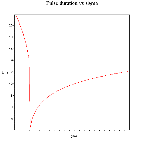
plot([seq(par3[j], j=1 .. 99)],axes=boxed,labels=[`Sigma`, `tp, fs`],title=`Pulse duration vs sigma`);
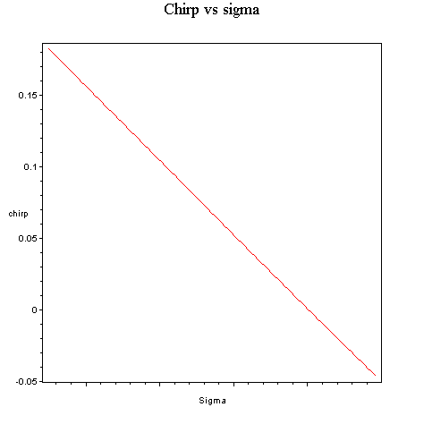
plot([seq(par4[j], j=1 .. 99)],axes=boxed,labels=[`Sigma`, `chirp`],title=`Chirp vs sigma`);
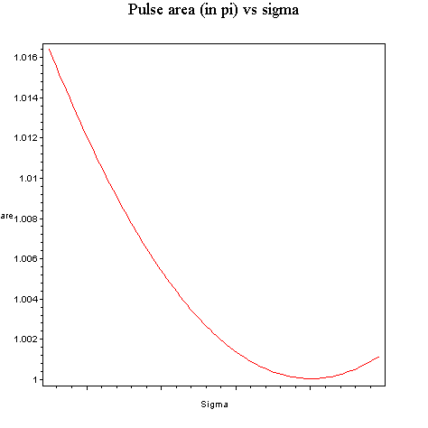
plot([seq(par5[j], j=1 .. 99)],axes=boxed,labels=[`Sigma`, `area`],title=`Pulse area (in pi) vs sigma`);

> sigma := 'sigma':
lambda := 'lambda':
par5 := array(1..40):
i := 1:
for lambda from 0.1 to 0.425 by 0.0125 do par5[i] :=
[lambda,Re(evalf(subs({beta=0.26,sigma=0.14},disp_2)))]:
i:=i+1: od:
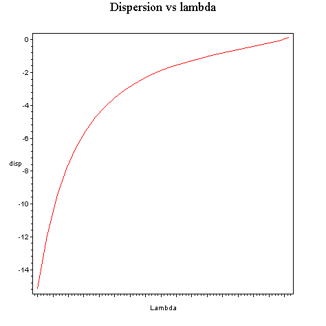
plot([seq(par5[i], i=1 .. 27)],axes=boxed,labels=[`Lambda`, `disp`],title=`Dispersion vs lambda`)

sigma := 'sigma':
lambda := 'lambda':
par6 := array(1..101):
j := 1:
for s from 0.01 to 0.1 by 0.0009 do par6[j] :=
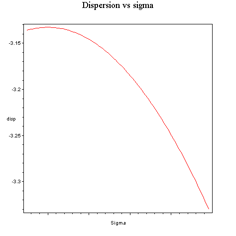
[s,Re(evalf(subs(lambda=0.2,subs({beta=0.26,sigma=s},disp_2))))]:
j:=j+1: od:

plot([seq(par6[j], j=1 .. 99)],axes=boxed,labels=[`Sigma`, `disp`],title=`Dispersion vs sigma`);

In the conclusion, the combined action of the Kerr-lensing, self-phase modulation, group-velocity dispersion and coherent absorption causes the formation of the sech-shaped pulse with p - area or chirped pulse with variable area. The duration of the chirped pulse in this case is close to the fundamental limit and can be controlled by the variation of the Kerr-lensing parameter or the relative mode radius in the active medium and absorber.