Capacity Allocation

Dynamic Capacity expansion problem

How should the plant capacity be decided? Typically demand for the product plays the deciding role.

Problem:
If a new plant is constructed with a capacity short of the actual demand, one cannot satisfy the demand and thus looses out on opportunity. On the other hand, if the plant is built with excess capacity, then besides under-utilization of capacity, capital also gets blocked. Hence, there is need for proper planning of capacity.
 

Goals of Capacity Planning

1. Maximize Market Share
2. Minimize under-utilization

Demand for a Product

The demand for a product could be ever increasing, as shown in the figure. In order to match demand, plant capacity may be expanded as shown, in discrete units, over time.

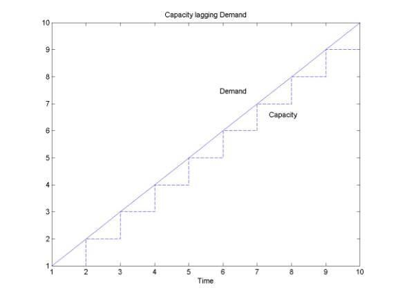
Figure 1 The Capacity Planning Problem

Analysis

Considerations

1. The demand for a product has been modeled as ever-increasing.
2. The capacity is expanded not continuously, but periodically. Let  represent the period of time after which capacity is expanded. Let  represent the annual increase in demand per time unit. Thus, in each time period of length , the capacity is expanded by  units per time period.
3. The principle of Time Value of Money notes that same unit of money is worth more today than in the future, since money with you today gives you the freedom to utilize it in a productive activity. Money obtained in the future is effectively blocked capital. This aspect is represented mathematically by an exponentially falling 'value' of money. Let  represents the annual discount rate. Implication:  unit of money obtained today is only worth  after  years.
4. Inflation effects Inflation is the rise in prices of commodities. Hence, over time the Purchasing Power of a unit of money decreases. Hence, a rupee now is worth less in the future due to inflation. Using a similar model to the above, we can get the actual value of a rupee after  years as  where  represents the Inflation rate. Alternately, the analysis can be performed for money in real terms. By definition, Real Money is money adjusted for inflation. For example, if a commodity was sold for Rs 10 a year earlier, and today costs Rs 11, then inflation rate = 10%. Hence, the rupee today is worth less than it was a year before due to general price rise. Thus, in real terms the rupee today (the nominal value) is worth  (the real value) where  is the inflation rate. Thus, as time passes, a rupee looses value at a yearly rate of where  is the annual discount rate and  is the inflation rate. In the rest of this discussion, money is considered to be in real terms, i.e it devalues at a yearly rate of . Alternately,  can be substituted for  to work with nominal money.
5. The Cost of a new Plant The cost incurred in setting up a plant is regarded as Fixed Cost. Typically, as larger plants - more capacity - are designed, the cost per unit capacity declines. This characteristic yields a decreasing slope curve. Let  represent the cost in setting up a plant of capacity . The curve can be represented mathematically by .
6. Parameter Values How are these parameters estimated?  is the cost of setting up a plant of capacity unit. In order to determine , consider the following. What is the cost involved in doubling the current capacity of a plant? Typically, this value can be estimated by plant designers. If the above model is correct, the plant with double capacity will cost as much as the existing one. Interestingly, this ratio is independent of the current capacity. From the estimate provided by the plant designer, the value of  can be estimated.

In order to meet the demand, let us assume that a plant of capacity  per year, is added after every  time period. This carries a cost of . Hence, the total cost incurred, now and in the future is given by Total Cost = 

The optimal duration of time  can be found from  which yields for optimal value 

Example: and . Find the Optimal time period  and the corresponding cost per period given  units increase per time period as the demand. The annual discount rate is . The graph of  can be used to quickly solve for .
 

Figure 2 Graph for determining optimum X

Hence, since at , we have , solve for  using , which yields   years (since  is the annual discount rate). Further Plant capacity  units and the cost of setting up plant is  million.
 

Learning Curves

As experience is gained with the production of a particular product by an individual or a firm, the production process becomes more efficient.

Factors contributing to learning

1. Individual workers' skill improves.
2. Improvement in production methods.
3. Tools and machines may change with reliability and efficiency improvements.
4. Better product design.
5. Improved production scheduling and Inventory control.
6. Better organization of work place.

Let  be the number of hours required to produce the  unit. From empirical studies,  can be characterized as .  is simply the time required to produce the first unit. In order to estimate  consider the time required to produce the  unit compared to the time needed to produce the .

This ratio is typically used to characterize the learning curve. For example, a  learning curve implies that the  unit is produced in  of the time it takes to produce the  unit.
 

Experience Curves

measure the effect that accumulated experience in the production of a product or a family has on overall cost and price. Typically, as more experience is gained, the cost of production per unit decreases. This trend has been witnessed in nascent industries undergoing major changes like the IC industry -- the cost per unit is seen to fall exponentially. Hence due consideration must be given to falling per unit cost in planning for the future.
 

Forecasting

Characteristics of Forecasts

1. They are usually WRONG. Thus, planning systems should be sufficiently robust to react to unanticipated forecasting errors.
2. A good forecast is more than a number. It is rather a range with some statistical significance.
3. Aggregate forecasts are more accurate, as errors cancel out. Hence it is more likely that the cumulative demand forecast of the entire product range is more accurate than forecasts for individual products.
4. The larger the forecast horizon, the less accurate the forecast.