About DSR*
The
Dynamic Source Routing protocol (DSR) is a simple and efficient routing
protocol designed specifically for use in multi-hop wireless ad hoc networks of
mobile nodes. DSR allows the network to
be completely self-organizing and self-configuring, without the need for any
existing network infrastructure or administration. The protocol is composed of the two main
mechanisms of "Route Discovery" and "Route Maintenance",
which work together to allow nodes to discover and maintain source routes to
arbitrary destinations in the ad hoc network.
The use of source routing allows packet routing to be trivially
loop-free, avoids the need for up-to-date routing information in the intermediate
nodes through which packets are forwarded, and allows nodes forwarding or
overhearing packets to cache the routing information in them for their own
future use. All aspects of the protocol operate entirely on-demand, allowing
the routing packet overhead of DSR to scale automatically to only that needed
to react to changes in the routes currently in use.
The DSR
protocol is designed for mobile ad hoc networks with up to around two hundred
nodes, and is designed to cope with relatively high rates of mobility.
Writing Wireless Simulation Scripts in NS
One needs to do a few more steps when writing a script for wireless networks in NS than for wired networks. These additional steps are listed below:
# create a flat topology in a 670m x 670m area
set topo [new
Topography]
$topo load_flatgrid
670 670
# nam trace
set namtrace [open
demo.nam w]
$ns
namtrace-all-wireless $namtrace 670 670
#create God
set god [create-god 3]
$ns at 900.00 “$god setdist 2 3 1”
# Define how a mobile node is configured
$ns node-config
\
-adhocRouting DSR \
-llType LL \
-macType Mac/802_11 \
-ifqLen 50 \
-ifqType Queue/DropTail/PriQueue \
-antType Antenna/OmniAntenna \
-propType Propagation/TwoRayGround \
-phyType Phy/WirelessPhy \
-channelType Channel/WirelessChannel \
-topoInstance $topo
-agentTrace ON \
-routerTrace OFF \
-macTrace OFF
Approach used in simulations
The following diagram explains flow of the scripts written for simulation
Supporting scene & traffic
generation scripts are used in addition to the basic script. NS produces two trace
files. One is used with Tracegraph & other with
Aims
The following are the goals of the project:
- simulating hidden node problem (RTS/CTS)
- simulating bandwidth limitation
- simulating DSR with 3 nodes (static)
- simulating DSR with 3 nodes (mobile)
- simulating DSR with 50 nodes (10 active connections)
- simulating DSR with 50 nodes (20 active connections)
1. Hidden node problem
Hidden node problem (see
Appendix) is simulated by starting two constant bit rate (cbr) traffic directed
at a single node at the same time.
…
$cbr_(0) attach-agent $udp_(0)
$ns_ connect $udp_(0) $sink0
$ns_ at 1.00 "$cbr_(0) start"
…
…
$ns_ connect $udp_(1) $sink0
$ns_ at 1.00 "$cbr_(1) start"
Excerpt from trace file:
…
s 1.007734320 _0_ MAC --- 0 RTS 44 [4fe 1 0 0]
r 1.008086987 _1_ MAC --- 0 RTS 44 [4fe 1 0 0]
s 1.008096987 _1_ MAC --- 0 CTS 38 [3c4 0 0 0]
r 1.008401654 _0_ MAC --- 0 CTS 38 [3c4 0 0 0]
s 1.008411654 _0_ MAC --- 0 ARP 80 [13a 1 0 806] ------- [REPLY 0/0
1/1]
r 1.009052320 _1_ MAC --- 0 ARP 28 [13a 1 0 806] ------- [REPLY 0/0
1/1]
s 1.009062320 _1_ MAC --- 0 ACK 38 [0 0 0 0]
r 1.009366987 _0_ MAC --- 0 ACK 38 [0 0 0 0]
...
The trace file shows node0 sending RTS to node1 which in turn sends a CTS. Node0 then sends an ARP packet to node1 which acknowledges the same. 3c4 represents the time expected to complete the following transmission including ACK. During this period no other node in the vicinity of node1 (except node0) would send any data.
2. Bandwidth Limitation
The next simulation shows how to limit physical bandwidth of an ad-hoc wireless LAN. One needs to add only a single line for the desired effect. e.g. for limiting bandwidth to 1Mbps one should add the following line:
…
Phy/WirelessPhy set bandwidth_ 1e6
# create
simulator instance
set ns_ [new Simulator]
…
The effect of above line can be shown with the help of
following graph:
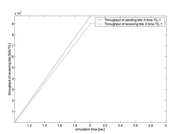
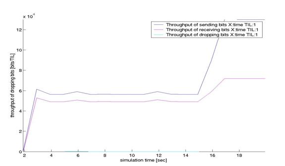
3. DSR with 3 nodes (static)
This simulation deals with light
load scenario where only 3 nodes are present and are exchanging data at cbr.
These nodes are static i.e. they do not move from their positions. Throughput
is shown below:
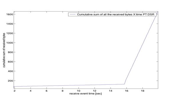
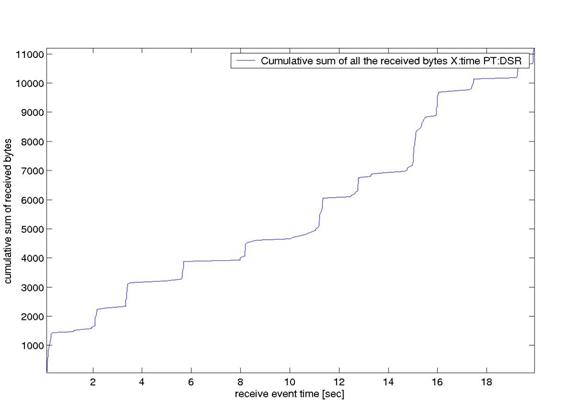
The following graph shows the cumulative sum (in bytes) of DSR packets exchanged.
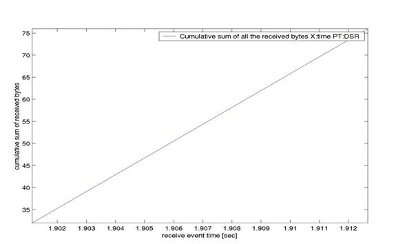
Since nodes are static, DSR packets are sent only during the
initial part of simulation.
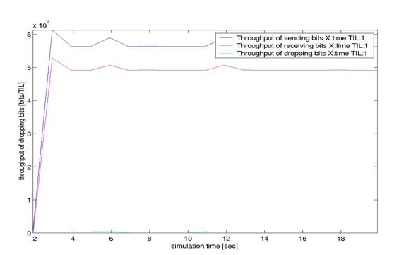
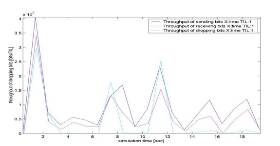
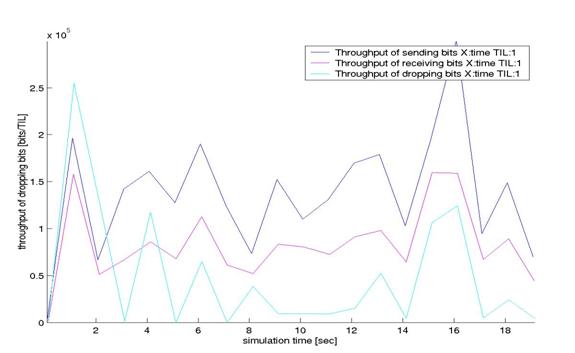
4. DSR with 3 nodes (mobile)
This is a slight modification
from the previous simulation in the sense that now the nodes are mobile.
Throughput of sending bits increases around 15s. This is so because now node2 receives data from node0 via node1. So packets are being received & sent twice.
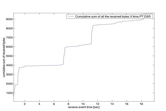
The DSR packets are continuously exchanged now as the nodes change their position especially in the latter part of simulation. Also, now around 1600 bytes of DSR data is being exchanged compared to just 75 bytes in static environment.
5. DSR with 50 nodes (10 active connections)
The rest two simulations are
illustrations of heavy load scenarios where 50 mobile nodes exchange data with
each other. In this script only 10 connections are active during the simulation
period. The traffic and scene files are recreated from ~ns/tcl/mobility/scene/
A maximum data rate of around
4x105 bits/s is achieved while around 9500 bytes of DSR data flows
through the network.
6. DSR with 50 nodes (20 active connections)
Now 20 connections are active
instead of 10. The following two graphs show a drop in peak throughput though
average throughput has increased but now more DSR data is being exchanged for
discovering & maintaining routes.
Comparison of last two simulations
Here are statistics of last two simulations.
- 50 nodes with 10 active connections
Simulation
length in seconds: 19.49670212
Number
of nodes: 50
Number
of sending nodes: 41
Number
of receiving nodes: 50
Number
of generated packets: 2295
Number
of sent packets: 2283
Number
of forwarded packets: 0
Number
of dropped packets: 810
Number
of lost packets: 0
Minimal
packet size: 28
Maximal
packet size: 612
Average
packet size: 82.5206
Number
of sent bytes: 231830
Number
of forwarded bytes: 0
Number
of dropped bytes: 103914
- 50 nodes with 20 active connections
Simulation
length in seconds: 19.84457401
Number
of nodes: 50
Number
of sending nodes: 47
Number
of receiving nodes: 50
Number
of generated packets: 3481
Number
of sent packets: 3414
Number
of forwarded packets: 0
Number
of dropped packets: 1206
Number
of lost packets: 0
Minimal
packet size: 28
Maximal
packet size: 644
Average
packet size: 83.0361
Number
of sent bytes: 359450
Number
of forwarded bytes: 0
Number
of dropped bytes: 135396
From the above statistics, it is clear that though data flow has increased by 50% the drop rate has only increased by 30%. So, performance of DSR has improved as more data flowed through the network.
Possible bug in NS
Study of trace files revealed that there might be a bug in NS. Following extract is an example:
s 1.005328986
_0_ RTR --- 1 DSR 32 [0 0 0 0] -------
[0:255 1:255 32 0] 1 [1 1] [0 1 0 0->0] [0 0 0 0->0]
s 1.005403986
_0_ MAC --- 1 DSR 84 [0 ffffffff 0 800]
------- [0:255 1:255 32 0] 1 [1 1] [0 1 0 0->0] [0 0 0 0->0]
r 1.006076652
_1_ MAC --- 1 DSR 32 [0 ffffffff 0 800]
------- [0:255 1:255 32 0] 1 [1 1] [0 1 0 0->0] [0 0 0 0->0]
r 1.006101652
_1_ RTR --- 1 DSR 32 [0 ffffffff 0 800]
------- [0:255 1:255 32 0] 1 [1 1] [0 1 0 0->0] [0 0 0 0->0]
In the above trace extract,
routing agent of node0 sends 32 bytes of DSR data to MAC layer. The MAC agent
adds 52 bytes of header and sends 84 bytes to node1. Now, instead of receiving
84 bytes at MAC layer, node1 receives only 32 bytes i.e. without 52 bytes
header. Though, MAC agent correctly delivers 32 bytes to routing agent of
node1.
Conclusion
As is evident from above simulations that dynamic source routing adapts quickly to routing
changes when node movement is frequent, yet requires little or no overhead
during periods in which nodes move less frequently. Though DSR overhead
increases when traffic is heavy or number of nodes are more but this should
still be less compared to distance vector protocols like DSDV where a complete
picture of the whole network is present at every node even though it might not
require it.
Appendix
ACK – Acknowledgement
CBR – Constant bit rate
CTS – Clear to
send
DSR – Dynamic Source Routing
Hidden node problem

Here nodes A & C are within
transmission range of B but cannot hear each other. Now, A starts sending data
to B. Since C is out of A’s transmission range, it senses the medium as free
and starts sending data to B. This results in collision at B. A is hidden from C and vice-versa.
NS
Network simulator, current version ns-2.1b9a can be downloaded from www.isi.edu/nsnam/dist
RTS – Request to send
Tracegraph
Tracegraph is a tool developed by Jaroslaw Malek([email protected]). This tool takes trace files outputted by NS as input and can be used for plotting various graphs like throughput, jitter, delays etc. It uses MATLAB libraries. It is available for download at www.geocities.com/tracegraph
References
- www.isi.edu/nsnam/ns
- The
NS manual,
- NS by example by Jae Chung and Mark Claypool (available at www.wpi.edu)
- Marc Greis’s tutorial web pages (available at ~ns/ns-tutorial)
- Mobile
Communications, Jochen H Schiller, Pearson Education
- NS users mailing list ([email protected])
- Tracegraph (www.geocities.com/tracegraph)