Simulating complex systems
Chalmers university of technology
Mahiar Hamedi, [email protected] 2000 06 05
Kinetic Monte Carlo simulations for growth on Al (111) surfaces and 3
dimensional low temperature structures
Growth of
islands on Al(111) resulting from diffusion at different temperatures in the
range 0-300 K has been studied, using KMC simulations.
KMC simulations have also been used simulating 3d fractal growth at low
temperatures.
Transition-state
theory (TST)
Growth is
a non-equilibrium phenomenon that involves macroscopic timescales. The most
straightforward way of addressing dynamical problems in materials is to
integrate Newton's equations for the particles of the system, this is called
molecular dynamics for atomic and molecular dynamics. The integration time step
in molecular dynamics must be typically as small as 1 fs to resolve the atomic
motion. This limits the possibility to access the timescales relevant for
growth. Molecular dynamics can be applied successfully in the study of single
atomic steps occurring in the growth, but the growth process as a whole must be
addressed elsehow.
The
computational complexity involved in transferring the f-second dynamics of
atoms to the seconds of growth experiments can be enormously reduced by
realizing that the adatoms reside in their binding sites and only rarely jump
to another site. If the time between the jump events is sufficiently long for
equilibriuim to be established, a statical-mechanical approach to the jump
frequency is justified.
TST yields from canonical distribution the rate for a system to go between two
states separated by a potential energy barrier. A typical example is an adatom
in the saddle point between two adjacent surface lattice sites.
Consider
a two state problem consisting of the initial state A and the final state B
divided by the transition state T. Making use of the assumption of canonical
ensemble it is possible to derive an expression for the rate at which the
infinite heat bath pushes the atom at site A above the barrier to site B. In
TST the atom changes state from A to B whenever the atom is located in a small
region around the transition state and moving towards site B. Now assume that
the atom is somewhere to the left of the transition state as in the figure
below
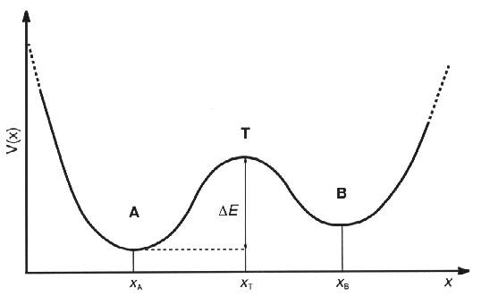
Fig 1. Example on typical
potentials for an atom as a function of space variable x
The
probability of finding the atom in a small region D x of the transition state x0 is
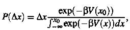 (1)
(1)
Where
b =1/kT. The upper limit of
the normalization integral in the domianator expresses the assumption that the
atom resides in site A initially. Likewise, the probability density for the
atom having the velocity v is
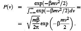 (2)
(2)
Within a
short time intervall D t the atom with
(positive) velocity v will enter site B provided that D x i smaller than vD t. The total probability that the atom can jump from site A to site B
can be written as
![]() (3)
(3)
where v A® B is the transition rate. Using equations (1) and (2)
we get
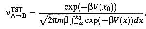 (4)
(4)
Thus the
problem reduces to solving the integral in the denominator of equation (4). If
V(x0) is much larger than kT, V(x) can be replaced with its expansion to second
order. The expression then becomes
![]() (5)
(5)
Where vA
is the harmonic vibration frequency of V(x) at site A, and D E is the diffusion barrier.
In experimental studies of single-atom diffusion on surface lattices, the
measured quantity is usually the diffusion constant D, which is defined through
the time dependence of the mean-squared displacement
![]() (6)
(6)
where a is the dimensionality of the motion. The diffusion
coefficient is related to the transition rate according to
![]() (7)
(7)
where g is the symmetry factor of the lattice (for example 3/4
for (111) surfaces), and l is the jump length.
VA in
equation 5 is referred to as the attempt frequency of the atom trying to
escape, succeeding with the rate vA® B. However vA
originates from the normalization integral of eq. (1) and does not have
anything to do with the actual motion of the atom.
Generalization
to the many body formulation of TST
Generalization
of the above argument to a system with N particles in 3D is straightforward and
yields
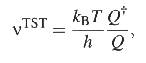 (8)
(8)
where h
is Planck's constant and Q denotes the classical partition functions of the
initial and transition states, respectivly given by
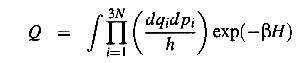 (9)
(9)
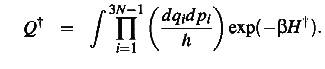 (10)
(10)
here the
H:s denote the Hamiltionians of the system in two states and {q,p} is any set
of generalized coordinates for the N-body system. At the transition state q3N
and p3N are the generalized coordinate and momentum along the reaction
coordinate. I.e the path in 3N-dimensional space that connect the initial and
final state. These are not included in Q-cross due to the constraints that the
system should be close to the transition state and moving towards the final
state.
The
integrals of eq. (9) and (10) can be calculated using the harmonic
approximation, which leads to the frequency-product formula
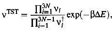 (11)
(11)
here the
vi:s are the harmonic vibration frequencies if the potential energy in the
initial and transition states, respectively. Setting N=1 which means that the
vibrational frequencies not related to changes in the adatom position are
assumed to cancel out, we get
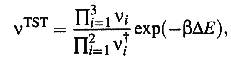 (12)
(12)
The
KMC algorithm
Given the
process rates from TST, a Kinetic Monte Carlo (KMC) simulation of the time
evolution is done in these steps
- Assume an initial
configuration for the system
- Create a list containing
all N possible reaction events j together from their calculated rates from
eq. (5) or (12) depending on the dimensions of the simulation.
- Pick an event in the
created list at random with the probability of choosing process j given by
4) increment clock by
5) Go to
step 2
KMC simulations
for Al(111) surfaces
The
characteristics of the Al(111) surface
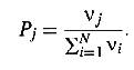
On the topmost
layer of a closed pack fcc (111) Al surface several diffusion processes can
occur. In the figure below each process is characterized by a letter (T for
terrace, k for kink, and C for corner) and a subscript that indicates the
number of in layer nearest neighbours before and after the jump. The processes
can take place at both A-steps with a {100} microfact and B-steps with a {111}
microfact.
Fig 2. Picture of different types
of possible processes
These
are the activation energies used in the simulation (see software). These values
are based upon semi-empirical results.
|
Process |
Symbol |
Diffusion
barrier (eV) A-step
, B-step |
|
Terrace
diffusion |
T 0® 0 |
0.04 |
|
Attachment |
- |
0.01 |
|
Dimer
Diffusion |
- |
0.13 |
|
Corner
flipping |
C 1® 1 |
0.18 ,
0.22 |
|
Corner
diffusion |
C 1® ³ 2 |
0.05 ,
0.19 |
|
Corner
crossing |
C 2® 1 |
0.33 ,
0.30 |
|
Corner
breaking |
C 3® 1 |
0.59 , 0.60 |
|
Edge
diffusion |
E2® 2 |
0.31 ,
0.26 |
|
Kink
breaking |
E3® ³ 2 |
0.42 ,
0.38 |
Choosing the
attempt frequency vA to be typically 10^13 in eq. (5) (motivated from TST, where vA originates from
the denominator of eq 1), we can compute the transition rate for each described
process with it's given energy barrier as a function of temperature. The result
is depicted in the figure3.
Fig 3. Each curve depicts the
transition rate for one process as a function of temperature. All curves start
from zero each increasing rapidly at the ”activation temperature” for the
process
Here we
can see that the transition rates for different processes start increasing
rapidly from near zero, at distinct temperatures. These temperatures can be
regarded as activation temperatures for the given processes. The figure 4 shows
the activation energies for possible processes
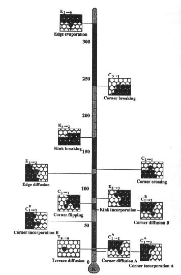
Fig 4. The activation energies for each process [1].
For example corner incorporation B is active for temperatures above 50 K
Choosing
the temperature high enough for the process corner incorporation to be active
the atoms can form arrangements of small clusters on a hexagonal (111) surface.
Clusters with four or more atoms usually tend to assume a compact form on open
surfaces for temperature intervals below the activation temperature of corner
breaking. The formation of a cluster usually proceeds by the attachment of a
single adatom forming tetramers, pentamers, hexamers, octamers and so on. The
figure below shows the geometry of small atomic clusters
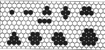
Fig 5. Example on different cluster
formations
As atoms
are induced on the surface from other layers the clusters start growing to form
islands. The shapes of these islands are dependent on the temperature and have been studied using KMC simulations.
The
Al(111) KMC computer simulation
Computer
simulations for the Al(111) surface has been made using the described KMC
algorithm (see section software download) and the given energy values. The
parameters in the simulation are Temperature, size of fcc site and A/B symmetry
(if A/B steps should be separated).
Several
interesting results are seen from the simulations. At low temperatures (60 K)
where only the processes terrace diffusion, attachment and corner diffusion are
active the islands grow in a star-like fashion in three preferential
directions, namely perpendicular to A steps. These so called dendrites have
been simulated with the KMC simulation [2] and can be seen to the right in figure 6.
The left picture shows the growth result for the same temperature but without
inclusion of the A/B symmetry (same energy levels for both A and B steps). The
result is here instead a random fractal.
The explanation is the anisotropy in corner diffusion i.e the process for which
an atom moves from a corner site to an edge. The barrier for going to the B
step is 0.19-0.05=0.14 eV higher than that for the A step (see diffusion
barrier table above). Corner diffusion is thus dominated by the B step. It is
amazing that nothing more than this seemingly unimportant process is needed to
transform the growth morphology from random fractal islands to regular
dendrites.
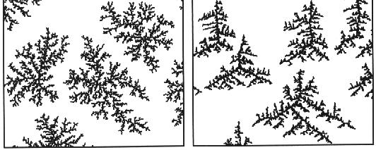
Fig 6. Growth simulated at
temperatures below 60 K [2]. The left
picture depicts growth without A/B symmetry.
Simulations are made by using KMC simulation software on unix stations at dep.
Of applied physics, chalmers.
Some
other KMC growth simulation have been made (with A/B symmetry included) at
different temperatures in the range 60-160 K. Note that other temperatures than
those included in the simulations depicted below would not give rise to any new
growth structures due to the distinct activation temperatures for each possible
diffusion process. For temperatures above 160 K, the processes kink breaking
and edge evaporation are active, and thus no island growth can take place.
The
simulation shows that for temperatures above 140 K compact islands are grown.
At these high temperatures kinetic effects are saturated due to the large space
of different diffusion processes and the thermodynamics rules. At 160 K the
structure is governed by the corner energetics.
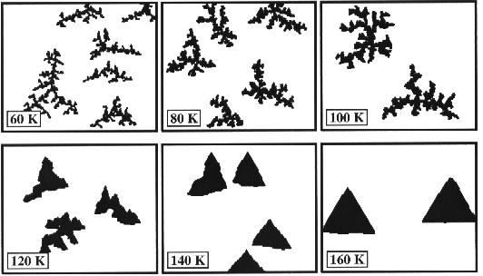
Fig 7. Growth at different temperatures with A/B symmetry [2].
KMC
simulations for 3-D growth
The many
body formulation of TST shows according to eq. (12) that the transition rates
for diffusion processes in 3-D follow the same exponential behaviour as used
above. Thus activation temperatures for each possible process in a 3-D growth
can be calculated using the energy barriers for these processes.
Since 3D
growth processes can not be bounded to a static lattice, there exists no
symmetries that can define an independent direction for the growth structure
(for example as for the dendrites), and the structure of stable growth shapes
is only dependent on the activated processes at the particular temperature.
Since
there exists a greater number of neighbouring sites for each atom in 3-D, the
number of different possible diffusion types is usually much more than for the
2D case. The space of different growth structures is therefore usually larger
in 3D.
Computer
simulation with KMC in 3-D
A
computer simulation on 3D growth has been made using the 3D software Maya.
Growth is simulated at low temperatures where only the two processes diffusion
and attachment are active. The simulation is performed using spherical particles
that move randomly in a confined 3d space until they collide and then attach.
The result of this simulation is identical to the KMC simulation for low
temperatures. The difference here is that there is no lattice with a structure
as the fcc structure for example. The result of such low temperature 3D growths
are fractals as in the 2D case with no isotropy. The result of a growth process
with 2000 particles are depicted below
at some different spatial angles
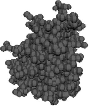
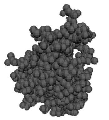
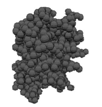
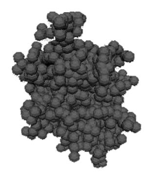
Fig 8. Growth simulated in 3d at
temperatures below 60 K.
The 3D
fractals are more tightly packed than those simulated on a surface. An explanation to this could be that the
particles do not move in discrete steps in a 3d lattice but continuous steps,
which decreases the possibility of particles to attach to border particles
(particles attached to only one other particle)
Growth at higher temperatures are harder to simulate using Maya and should be
simulated using a complete 3D KMC
simulation.
It is however very interesting to simulate such growth structures where several
processes can be active. One could for example think of simulating growth with certain
molecules in liquids with given temperature and characteristic activations
energies suitable for growth. The growth structure in such cases would be difficult
to predict theoretically as for the Al growth
demonstrated previously.
Software
/ download
The
fcc KMC simlation
A KMC
simulation software for the fcc structures in connection to this paper has been
created. The software is created in visual C++ and can be compiled on regular
PC computers.
The activation energies used are the ones described above. The main parameters
of interest are temperature, size of the lattice and the growth rate. With
different parameters figures similar to the ones in figure 7 can be generated.
The growth properties can be changed by changing the parameters at the
beginning of the file user.cpp. This file contains the complete program for the
KMC on fcc structures.
The project file can be downloaded here: VC-Project.ZIP
A compiled executable example of the program can be downloaded here Mahiar.zip. The following parameters used in this
simulation
Lattice size 150X150, Temp. 140 K, growth rate 0.0001 ml/s. Please note that
KMC simulations require large amounts of computation and will usually require
several hours of simulation time.
The 3d
simulation
The 3D
fractal growth is created in Maya’s Mel script. The script can be downloaded
here diff.zip (MEL script)
The maya scene decpicted in fig 10 can be downloaded here 3d_Diffusion_Scene.zip This scene can only be
viewed using the maya software.
References
[1] Alexander Bogicevic, Atom Dynamics and
Diffusion on Surfaces (1998)
[2] Staffan Ovesson, Diffusion, Nucleation, and Island
Growth in Metal-on-Metal Epitaxy, Licentiate Thesis, Department of Applied
Physics
Chalmers University of Technology
and Göteborg University (2000).