Mahiar Hamedi

 

Exercise 4, SOFM for 2d visualization of multidimensional distributions

Definition of the exercise

2. Apply your SOFM program to map at least two examples of high-dimensional distributions (for example using data for the application examples in Homework 2) to 2-d! Try to find a good solution for the visualization of your results! Discuss any problems that occur!

 

Background to the implementation

The SOFM algorithm was implemented in Matlab using the following parameters

 

 

 

Where a is the leaning rate,s  is the width of the neighbourhood function and the number of neurons used are n*n in a 2d mesh.

The neighbourhood function h is chosen as Gaussian distribution i.e.

 

 

where d is the distance between randomly chosen neuron and other neurons i.

 

 

Results, tested on wine data

The algorithm was tested on a wine data where 13 dimensional data is listed for wines from a district in Italy but with three from 3 different cultivars.

 

 

 

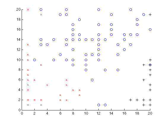
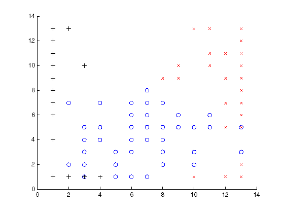
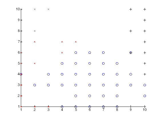
Figure 1.  Different  iterations of the SOFM with n=20, n=14 and n=10. Circles stars and plus symbolize the three different regions.

 

Figure 1 shows the SOFM visualization with  different n. The wine data from different districts are clearly grouped in the 2-d map. The result is already visible with 10x10 neurons.

 

 

The Matlab code

You can view the matlab code here:

 

%----------------------------------------------------------------------
% Author:       Mahiar Hamedi
% Description:  SOFM algorithm, for mapping wine data
%----------------------------------------------------------------------

%--- Variable definition and initialization
clear;

W=dlmread('wine_data.txt',',');
Nside=20;
N=Nside*Nside;          % Nr Neurons
sN=1000*log(sqrt(N));
dim=13;                 % Nr of data dimenstion
m=rand(N,dim);          %inititial constantly random distributed values for the modelvector
alpha=0;                %lerning rate f(t)
sigma=0;                %width of neighbourhood function f(t)

%create matrix with neuron positions
for i=1:N
   Npos(i,2) = mod(i-1,Nside)+1;
   Npos(i,1) = fix((i-1)/Nside)+1;
end

sW=size(W);
sW=sW(1);
% Normalize wine data
Wn = W(:,2:14);
Wn = Wn-ones(sW,1)*min(Wn);
for i=1:dim
   Wn(:,i) = Wn(:,i)/max(Wn(:,i));
end

%Iteraion loop
for t=0:6000
    % calculate alpha(t) and sigma(t)
    sigma=sqrt(N)*exp(-t/sN);
    alpha=0.1*exp(-t/1000);   
  
    %pick random neuron and find nearest data (similarity matching)
    x=Wn(ceil(rand*sW),:);
    
    n=0;
    Mint=1;
    for i = 1:N
      tn = norm(x-m(i,:));
      if tn < Mint
         n = i;
         Mint = tn;
      end 
    end
    Dpos = ones(N,1)*[ceil(n/Nside) mod(n,Nside)+1];
    n = abs(Npos-Dpos);
    n = n(:,1)+n(:,2);

    %calculate gaussian neighbourhood function
    h = exp(-(n.^2/(2*sigma^2)))*ones(1,dim);
    m = m + alpha*(h.*([ones(N,1)*x]-m));
   
    %display two dimensions of the neurons
    if mod(t,300)==1
        figure(1);
        plot(m(:,1),m(:,2),'.',m(:,1),m(:,2),'-');
        title(sprintf(' Nr iterations: %u',t))
        drawnow;
    end
end

% Similarity matching - Competitive Process
figure(3);
clf;
hold on;
for i=1:sW
   Mint = 1;

           for j = 1:N
              tn = norm(Wn(i,:)-m(j,:));
              if tn < Mint
                 Mint = tn;
                 d = j;
              end
           end
     
   y = mod(d,Nside)+1;
   x = ceil(d/Nside);
   if(W(i,1)==1)
       plot(x,y,'rx');
   end
   if(W(i,1)==2)
        plot(x,y,'bo');
   end
   if(W(i,1)==3)
        plot(x,y,'k+');
    end
end