Such posed, the problem is called Bolza’s problem. Special cases of it are: Lagrange’s problem (f=0) and Meyer’s problem (F=0). Special case of Lagrange’s problem is a Minimal Time problem (F=1).

Pontryagin’s Maximum Principle

Let’s introduce adjoined variables y₁...y_n, such that:

where H(x, y, u, t) – Hamilton’s function:

According to Pontryagin’s Maximum Principle, optimal control u* will deliver maximum to Hamilton’s function (necessary condition of optimality):

where: G – restrictions, imposed on control: u(t) Î G

In the absence of restrictions on control, maximum usually can be found from the condition:

Piecewise solutions

Variational methods described above assume continuity and differentiability of the optimal control (class C₁). In reality, the optimal control often does not have this property.

For example, consider the following example: rocket needs to reach point B from the point A in a minimal time. Also, at the start and finish rocket must have zero velocity, its acceleration is constant and external forces are absent. Optimal control in this case will be the following: through the first half of the trajectory rocket will accelerate toward point B, and during the second half it will slow down. Such control has a point of discontinuity in the middle of the trajectory.

Therefore, continuous solution, satisfying Pontryagin’s Principle, is not always optimal. Moreover, it may be not optimal even in the class of continuous functions.

Let’s assume that we have found a continuous solution, that satisfy Pontryagin’s Principle and border conditions. Let’s assume also that optimal control is discontinuous. Let’s consider control that is close enough to an optimal (discontinuous) but still is continuous and differentiable, and let it also satisfy the border conditions. Such control will be more optimal then the one found from Maximum Principle.

This seeming paradox can be explained in the following manner: Maximum Principle is satisfied by controls that are optimal (extremal) in some neighborhood. In out case, control that is close to optimal (discontinuous) is not an extremum: there always exists a control that is closer to the optimal and extremum is never achieved in the class of continuous functions.

In such cases, in practice, the solution is found in the class of piecewise-differentiable functions. Such control satisfies Pontryagin’s principle on each interval of continuity but may have points of discontinuity.

Finding optimal control

First, let’s consider finding of the optimal control in the class of differentiable functions. We know the initial state of the system. Let’s also assume that we know initial values of the adjoined variables. Optimal control at any moment can be determined from the state of the system through Pontryagin’s Principle. Then, solving together main and adjoined systems of differential equations (Cauchy problem), we can find the final state of the system.

Therefore, the problem is reduced to the finding such initial values for adjoined variables that deliver required final state to the system. In general case, this problem is resolved numerically and, if the dimension of the problem is significant, can be quite computationally intense.

Now let’s make transition to finding control in the class of piecewise-differentiable functions. Let’s assume that we know the number of discontinuity points n, the times of discontinuities t_i and states of the system u_i in these moments. Then, solving previous problem for each interval, we can obtain control that will be optimal for a given set {n, t_i, u_i}.

The problem is reduced to the optimization (in general case, numerical) of the parameters’ set {n, t_i, u_i}. At each step of the optimization we have to solve n+1 problems of finding optimal control in the class of differentiable functions in the way described above. Needless to say, this process could be quite taxing.

Movement of the rocket

In this section we will use the following assumptions:

- assume that rocket’s engines thrust and acceleration are predetermined

- assume certain physical model of the environment (we will use several of those)

We will be solving the following problem: given thrust program, what is the optimal pitch* program (under the assumptions of the given physical model) ?

Here we define optimal program as one that delivers the payload to the given altitude with given (usually, zero) vertical velocity and maximal horizontal velocity**.

(*) pitch is the angle between the main axis of the rocket and the local horizon.

(**) for those interested in Optimal Control Theory, note that for such problem, optimality could be defined in various ways – however the result will be the same.

Below, we will derive an optimal solution for several simplified physical models of the environment. Given the fact that any chosen model is just an approximation of the real environment, the control program that results from it will be, in fact, quasi-optimal.

Flat gravitational field

Consider application of the Maximum Principle on a simple example.

Let rocket move in a flat gravitational field.

System dynamics:

where:

a(t) – characteristic acceleration

q – pitch angle

Hamilton’s function:

Here and below: by y_x, y_y we designate adjoined variables corresponding to V_x, V_y, and by j_x, j_y – corresponding to x, y.

Applying Maximum Principle, obtain:

(1)

Adjoined system:

Easy to see that in this case, optimal program for a tangent of a pitch is fractional-linear:

Free coefficients are determined (less arbitrary multiplier) by the boundary conditions.

Problem of achieving given height

Let’s simplify the previous problem and instead of aiming at the certain point, require only achieving certain altitude. Then:

(2)

In this case, optimal program simplifies and becomes linear:

Central gravitational field

Let’s transition to rotating system of coordinates, linked to a center of the Earth and to the rocket (“orbital” system of coordinates). Introducing centrifugal and Coriolis accelerations:

(3)

Here: r – distance to the center of the Earth (r ≡ y+r₀); r₀ – Earth radius.

Solving together main and adjoined systems, determine optimal control from condition:

Aerodynamics – drag force

Consider optimal control for a simplified aerodynamic model, which accounts for a drag force (aerodynamic force vector is collinear to the velocity). This model does not account for a lift force and, consequently, applicable only when either angle of attack or aerodynamic quality are small.

Let’s write aerodynamic force as:

where:

q = ½rV² – dynamic pressure

C_x – aerodynamic drag coefficient

S – typical area

r₀ – air density at sea level (y=0)

b – exponential factor of air density reduction

Main and adjoined systems:

where:

As in previous example, solving together main and adjoined system, determine optimal control from the condition:

Aerodynamic model

In the general case (for non-zero angle of attack), full aerodynamic force can no longer be assumed collinear to the velocity vector. Problem of precise measurment of aerodynamic force is very difficult and for bodies of a complex shape can only be resolved through experiment (in wind tunnels). Solution is obtained in the form of experimental tables or approximating curves.

The following model is often used as an approximation. It satisfactory estimates aerodynamic force for relatively small (to ~15 degrees) AOA.

In “velocity” system of coordinates (linked to a velocity vector):

where:

a – angle of attack (angle between the axis of the rocket and velocity vector)

q – dynamic pressure

C_x – a/d drag coefficient

C_y – a/d lift coefficient

(*) Note that here we neglect viscose friction.

We will use trigonometric representation of this model in linked (to the body’s axes) system of coordinates:

(4)

where:

R_D, R_L - a/d force projections of the body’s axes (main and side)

S_D, S_L - body’s typical areas (frontal and side sections)

(**) Usually values of a/d coefficients are taken for the same area (wing), but here we will use two different areas: frontal section area (typical area for the drag force) and area of the side section (typical area of the lift force).

Easy to see that both representations are identical up to o(a²)

When the vehicle has an aerodynamic quality it becomes possible to control the lift force through change of AOA. As aerodynamic axis and thrust vector not necessary need to coincide – we have one more independent control variable:

c – angle between a/d axis of the vehicle and the horizon

As before, for the angle between the thrust vector and the horizon we will use notation q .

Aerodynamics – lift force

Therefore, for the chosen aerodynamic model, the system dynamics takes form:

(5)

where:

R_x= R_Dcosc – R_Lsinc = -q [ C_DS_Dcosa cosc + C_LS_Lsina sinc ]

R_y= R_Dsinc + R_Lcosc = -q [ C_DS_D cosa sinc - C_LS_L sina cosc ]

- a/d force projections on the axes of the main (orbital) system of coordinates.

Expressing AOA a through the pitch angle and velocity vector components, after substitutions and transformations, obtain:

(6)

where:

Note that the expression:

is closely related to the aerodynamic quality, which is defined as:

If there are no restrictions imposed on q and c, maximum of Hamiltonian corresponds to:

(7)

Therefore, the optimal control {q, c } satisfies:

where:

n – angle between the velocity vector and the horizon

We have obtained an interesting result:

The optimal direction fоr the aerodynamic axis of the vehicle is a bisector of the angle formed by the velocity and thrust vectors (8)

For the model (4) this relationship holds exactly. Besides, for rather broad class of aerodynamic models it holds up to о(a²).

Aerodynamics – lift force (restricted case)

In the previous chapter we assumed that the vehicle orientation c is arbitrary and does not depend on the direction of the thrust q. In many cases it is not true. For example, for a typical rocket thrust vector and vehicle axis must coincide (q = c). We will consider somewhat more general case: q = c + g ₀.

Let’s find the optimal control for this special case:

or, after transformations:

(9)

where:

Trigonometric equation (9) can be reduced to the algebraic equation of fourth power. Solving it, we can obtain optimal control q^*. Though equation of fourth power can be resolved in radicals (for example, by Ferro’s method), the solution formula is quite cumbersome. Simple method for its approximate solution is described below:

From general considerations, we can assume that optimal value q^* should not be too different from q₀– that is, Dq is small. Expanding series by Dq up to O(Dq), obtain:

where:

In the same way, using expansion up to O(Dq²) and solving quadratic equation, obtain more accurate approximation of Dq:

Aerodynamics – transonic velocities

Until now we have assumed that a/d coefficients are constant. In reality, if velocity is comparable to the speed of sound, coefficients strongly depend on the velocity. For example, the drag coefficient sharply increases in transonic interval and then reduces:

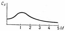
In general, dependence of a/d coefficients from the velocity is quite complex, strongly depends on the body’s shape and is determined through experiment (in aerodynamic tubes).

... in progress…

Aerodynamics – hypersonic velocities

At hypersonic velocities the pattern of dependence from AOA is changing. For example, lifting force becomes proportional a² (Newton).

... in progress…

Optimal thrust program

Until now, we assumed that the rocket’s thrust is predetermined. It is not always so. For a multistage rocket, if several stages are working simultaneously, the optimal thrust (throttling) has to be chosen.

To achieve the maximal characteristic velocity it is necessary that the stages work strictly consequently. However, this leads to smaller thrust and longer burn. Consequently, the gravitational losses increase. Moreover, for some rockets, the thrust of the first stage is not sufficient to lift the rocket from the launchpad. Simultaneous burn of the first and second stage is necessary.

Consider the optimal thrust program for the second stage (during the first stage burn). For this we need to introduce one more state variable: the mass.

where u – specific impulse

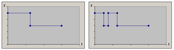
Note that Hamilton’s function is linear in thrust F. This means that Hamilton’s function maximum is delivered either by maximal or by minimal thrust value (depending on the sign of the expression at F). Therefore, optimal thrust program should consist of intervals of maximal and minimal thrust.

Analyzing the sign of the expression at F, it’s easy to see that, in absence of the a/d drag, the thrust of the second stage should be maximal at first, and then (from the certain moment and up to the first stage separation) – minimal (chart to the left).

If we introduce a/d drag, it is possible (however not necessary) that one another interval of minimal thrust will appear (chart to the right).

Note that:

We assume that engine’s specific impulse does not depend upon thrust value, i.e. depth of the throttling. It is not quite so. Usually, throttling engine down results in reduction of specific impulse. However, the conclusion that the optimal thrust level is either maximal or minimal still holds if the dependency of the specific impulse on throttling is sufficiently small.
These charts demonstrate the general form of the optimal program. Depending on mass/thrust characteristics of the rocket, any special case is possible. For example: second stage thrust may be maximal (or minimal) during all the first stage burn; “aerodynamic” interval of the minimal thrust may be absent; etc.
Theoretically, the restriction of the minimal thrust may be absent (F_min=0). However, as a rule, in reality, deep throttling (of complete turning off) of the engine is either not possible at all, or leads to substantial losses.
Naturally, the real thrust programs have more complex form (which, generally speaking, is a deviation from the mathematical optimality). Such complexity is due to the various restrictions of the engineering nature (see more in the section “Control restrictions”).

Control restrictions

... in progress…

Comparison of various programs

Summary table

The following table summarizes the elements of the system dynamics and the adjoined system for various control models. These elements were described with more details in the corresponding sections above.