Considerations Regarding The Kandoian & Sichak Formula

Considerations Regarding
The Kandoian & Sichak Formula

by Andrés Esteban de la Plaza

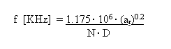
The formula given by Kandoian & Sichak to calculate the quarter-wave resonant frequency f of a coil in kilohertz is:

where a_r is the aspect ratio (H/D), N the number of turns and D the diameter if the coil in inches. According to K&S, agreement is within 10% of experimental values.

It may be shown that this formula may well be obtained considering only the distributed capacitance of the coil.

In his paper "TESLA COIL MYTHS" (Tesla Coils Builder Association -TCBA News, Volume 6, #3. 1987), Mr. William M. Colb deals with The Quarter-Wave Coil and explains the difference between electrical and physical length, and introduces de Kandoian & Sichak well known formula.
I will show in this paper that the K&S formula may be obtained considering only the distributed capacity of the coil (Medhurst's formula) combined with the usual tank formulas...

This distributed capacitance, due to the electrostatic effects of the coil’s winding may be obtained from the Medhurst’s work. Thus, according to Medhurst (Medhurst, R. G. "High Frequency resistance and self-capacitance of single-layer solenoids") the self-capacitance value is given by C[pF] = K· D, where the k parameter depends only on the length/diameter (aspect ratio) relationship, and D is the coil diameter in centimeters, thus C [pF] = k · D

Then, for common aspect ratios found in Tesla coils Þ 1 < a_r < 7 , we have the following table of k:

a_ratio	k
7.0	1.01
6.0	0.92
5.0	0.81
4.5	0.77
4.0	0.72
3.5	0.67
3.0	0.61
2.5	0.56
2.0	0.50
1.5	0.47
1.0	0.46

A regression analysis of this table will give the following function for k as a function of a_r:

k = 0.0965· a_r + 0.3408

but a better approximation is given by:

k = 0.1·a_r + 0.32.

On the other hand if we want a power form for the regression curve, instead of the linear one, then after some "number crunching" we will obtain:

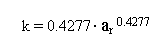
Thus the Medhurst formula may be written as:

C [pF] = k· D[in]·2.54

C [pF] = 0.4277· a_r ^0.4277·D[in]·2.54

C [pF] = 1.08636· a_r ^0.4277·D[in]

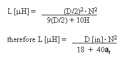
Now let’s continue with the Wheeler’s formula for the inductance of the coil:

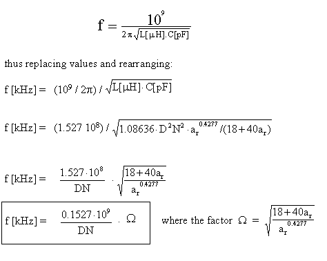
Now let’s calculate the resonant frequency using Wheeler & Medhurst:

Now let’s see if we can obtain a regression formula for W in the power form y = . Thus, we plot W for different a_r values, 0.5 < a_r < 10 , and obtain the following table:

a_r	W
0.5	7.14936
1.0	7.61577
1.5	8.09823
2.0	8.53567
2.5	8.92980
3.0	9.28768
3.5	9.61567
4.0	9.91881
4.5	10.20101
5.0	10.46534
5.5	10.71425
6.0	10.94970
7.0	11.38633
8.0	11.78508
9.0	12.15293
10.0	12.49505

The best regression is a power curve given by

W = 7.65464· a_r^0.19815

Now we replace this formula of W in the f [kHz] one, thus:

f [Hz] = 0.1527· 7.65464· 10^9·a_r^0.19815 / DN

f [Hz] = 1.16886· 10^9·a_r^0.19815 / DN

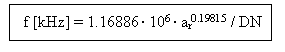
Now let’s compare this formula with the Kandoian & Sichak one:

What about the 1.16866 instead of 1.175?

Þthere’s only 0.523% difference...

What about the exponent 0.19815 instead of 0.2?

Þthere’s only 0.925% difference...

Should we conclude that both formulas are the same? I believe the answer is YES!

The approach taken has some interesting points we should consider:

We used the tank formula (f = 1/ ), the Wheeler’s formula for the inductance and the approximation of the capacitance of the coil as a distributed parameter...

[email protected]