 |
|
|
|
|
|
|
|
|
|
|
|
|
|
|
|
|
|
|
|
|
|
|
|
|
|
|
|
|
|
|
|
|
|
|
|
|
|
|
|
|
|
|
|
|
|
|
|
|
|
|
|
|
|
|
|
|
|
|
|
|
|
|
|
|
|
|
|
|
|
|
|
|
|
|
|
|
|
|
|
|
|
|
|
|
|
|
|
|
|
|
|
|
|
|
|
|
|
|
|
|
|
|
|
|
|
|
|
|
|
|
|
|
|
|
|
|
|
|
|
|
|
|
|
|
|
Capacity of Wireless Channels |
|
|
| Introduction : |
|
|
|
The interest in wireless communications has increased dramatically, as seen by growth of cellular telephony, personal communication systems, and indoor applications. This increased interest has brought more focus on the problems unique to the wireless environment. Including capacity limits due to spectrum availability. |
|
|
| Capacity limits dictate the maximum data rates that can be transmitted over wireless channels with small error probability. Shannon defined capacity as the mutual information maximized all over all possible input distributions. The significance of this mathematical construct was Shannon's code theorem and converse, which proved that a code did exist that could achieve a data rate close to capacity with negligible probability of error, and that any data rate higher than capacity could not be achieved without an error probability bounded away from zero. |
|
|
|
1. Capacity in AWGN |
|
|
|
 |
|
|
|
|
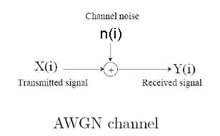
Consider a discrete-time additive white Gaussian noise (AWGN) channel with channel input/output relationship :
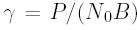
y[i] = x[i] + n[i], where x[i] is the channel input at time i, y[i] is the corresponding channel output, and n[i] is a white Gaussian noise random process. Assume a channel bandwidth B andtransmit power P. Thechannel SNR, the power in x[i] divided by the power in n[i], is constant and given by : |
|
|
|
 |
|
|
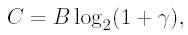
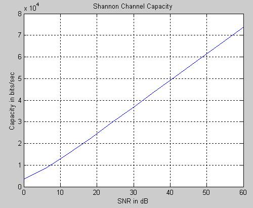
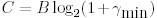
| Where N0is the power spectral density of the noise. The capacity of this channel is given by Shannon?s well-known formula : |
|
|
|
 |
|
|
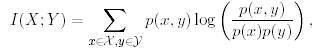
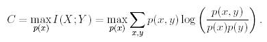
| Shannon's capacity can be defined as the maximum mutual information of a channel. Its significance comes from Shannon's coding theorem and converse, which show that capacity is the maximum error-free data rate a channel can support.The converse theorem shows that any code with rate R.> C has a probability of error bounded away from zero. The theorems are proved using the concept of mutual information between the input and output of a channel. For a memory-less time-invariant channel with random input x and random output y, the channel?s mutual information is defined as : |
|
|
|
 |
|
|
|
Shannon proved that channel capacity equals the mutual information of the channel maximized over all possible input distributions : |
|
|
|
 |
|
|
|
Shannon capacity is generally used as an upper bound on the data rates that can be achieved under real system constraints. At the time that Shannon developed his theory of information, data rates over standard telephone lines were on the order of 100 bps. Thus, it was believed that Shannon capacity, which predicted speeds of roughly 30 Kbps over the same telephone lines, was not a very useful bound for real systems. |
|
|
|
However, breakthroughs in hardware, modulation, and coding techniques have brought commercial modems of today very close to the speeds predicted by Shannon in the 1950s. In fact, modems can exceed this 30 Kbps Shannon limit on some telephone channels, but that is because transmission lines today are of better quality than in Shannon?s day and thus have a higher received power than that used in Shannon?s initial calculation. Traditional modems have a limitation on the data rate (maximum of 33.6 kbps) as determined by the Shannon formula. However, new modems, with a bit rate of 56 kbps are now in the market. These modems may be used only if one party is using digital signaling (such as Internet provider). They are asymmetrical in that the down loading is maximum 56kbps while the uploading is maximum of 33.6 kbps. |
|
|
|
 |
|
|
|
The figure shows the relation between SNR in dB and the channel capacity in bits/sec at band width 3700 Hz which is typically for the band width of a twisted-pair telephone line channel. |
|
|
|
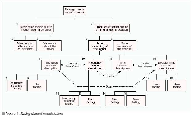
A very important issue in practical wireless networks, is the presence of multi-path fading . In a wireless network, due to the physical environment, the electromagnetic waves travel to receivers along a multitude of paths. Depending on the frequency bandwidth used, and how fast the environment changes, the fading can be divided into two cases: |
|
|
|
1. If the bandwidth W of the signal is much smaller than the channel coherence bandwidth , i.e., W<<Bcoh, then fading is roughly equal across the entire signal bandwidth, then the channel is frequency non-selective or flat fading. This means that the channel only has a multiplicative effect on the signal. |
|
|
|
 |
|
|
2. If on the other hand |
|
|
|
|
|
|
the receiver will get several resolvable signal components, the channel amplitude varies widely across the signal bandwidth and such a channel is called frequency selective. |
|
|
|
 |
|
|
|
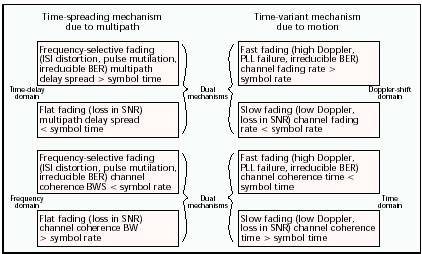
When viewed in the time-delay domain, a channel is said to exhibit frequency-selective fading if Tm > Ts (the delay time is greater than the symbol time). This condition occurs whenever the received multipath components of a symbol extend beyond the symbol?s time duration, thus causing channel-induced intersymbol interference (ISI). |
|
|
|
Viewed in the time-delay domain, a channel is said to exhibit frequency-nonselective or flat fading if Tm< Ts. In this case, all of the received multipath components of a symbol arrive within the symbol time duration; hence, the components are not resolvable. |
|
|
|
Here, there is no channel-induced ISI distortion, since the signal time spreading does not result in significant overlap among neighboring received symbols. There is still performance degradation since the unresolvable phasor components can add up destructively to yield a substantial reduction in signal-to-noise ratio (SNR). |
|
|
|
When viewed in the frequency domain, a channel is referred to as frequency-selective if f0 < 1/Ts = W, where the symbol rate, 1/Ts is nominally taken to be equal to the signal bandwidth W. Flat fading degradation occurs whenever f0 >; W. Here, all of the signal?s spectral components will be affected by the channel in a similar manner (e.g., fading or no fading). In order to avoid ISI distortion caused by frequency-selective fading, the channel must be made to exhibit flat fading by ensuring that the coherence bandwidth exceeds the signaling rate. |
|
|
|
When viewed in the time domain, a channel is referred to as fast fading whenever T0< Ts, where T0 is the channel coherence time and Ts is the symbol time. Fast fading describes a condition where the time duration for which the channel behaves in a correlated manner is short compared to the time duration of a symbol. Therefore, it can be expected that the fading character of the channel will change several times during the time a symbol is propagating. This leads to distortion of the baseband pulse shape, because the received signal?s components are not all highly correlated throughout time. Hence, fast fading can cause the baseband pulse to be distorted, resulting in a loss of SNR that often yields an irreducible error rate. Such distorted pulses typically cause synchronization problems, such as failure of phase-locked-loop (PLL) receivers. |
|
|
|
Viewed in the time domain, a channel is generally referred to as introducing slow fading if T0 > Ts. Here, the time duration for which the channel behaves in a correlated manner is long compared to the symbol time. Thus, one can expect the channel state to remain virtually unchanged during the time a symbol is transmitted. |
|
|
|
 |
|
|
|
Small-scale fading: mechanism, degradation categories, and effects |
|
|
|
2. Capacity of Flat-Fading Channels |
|
|
|
Depends on what is known about the channel. |
|
|
|
Four cases: |
|
|
|
1) Nothing known; |
|
|
|
2) Fading statistics known; |
|
|
|
3) Fade value known at receiver; |
|
|
|
4) Fade value known at transmitter and receiver. |
|
|
|
Case 1 : Unknown Fading : |
|
|
|
 |
|
bps, |
|
|
|
|
|
where g min is the minimum fade SNR . For many flat-fading channels |
|
|
|
= 0, leading to a Shannon capacity of zero. |
|
|
|
 |
|
|
|
|
|
|
|
|
|
Case 2 : Fading Statistics Known : |
|
|
|
Difficult to compute: only known results are for Finite State Markov channels, Rayleigh fading channels, and block fading. |
|
|
|
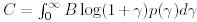
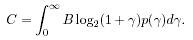
Case 3 : Fading Known at the Receiver : |
|
|
|
 |
|
|
|
bps, |
|
|
|
|
|
where |
|
|
|
;is the distribution of the fading SNR . |
|
|
|
 |
|
|
|
|
|
|
|
|
|
? By Jensen?s inequality this capacity always less than that of an AWGN channel. |
|
|
|
? ?Average? capacity formula, but transmission rate is fixed. |
|
|
|
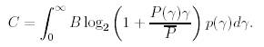
Case 4 : Capacity with Fading Known at Transmitter and Receiver |
|
|
|
For fixed transmit power, same capacity as when only receiver knows fading. |
|
|
|
Transmit power as well as rate can be adapted. Under variable rate and power |
|
|
|
 |
|
|
C = |
|
|
|
|
|
|
where S(g) is power adaptation. |
|
|
|
2.1 Channel Distribution Information |
|
|
|
We first consider the case where the channel gain distribution p(g) or, equivalently, the distribution of SNR p(g) is known to the transmitter and receiver. Fading correlation introduces channel memory, in which case the capacity-achieving input distribution is found by optimizing over input blocks, which makes finding the solution even more difficult. |
|
|
|
The capacity-achieving input distribution and corresponding fading channel capacity under CDI is known for two specific models of interest : Rayleigh fading channels and Finite State Markov Channel (FSMCs). |
|
|
|
In Rayleigh fading the channel power gain is exponential and changes independently with each channel use. FSMC approximates the fading correlation as a Markov process. While the Markov nature of the fading dictates that the fading at a given time depends only on fading at the previous time sample. |
|
|
|
Capacity of the FSMC depends on the limiting distribution of the channel conditioned on all past inputs and outputs, which can be computed recursively. As with the Rayleigh fading channel, the complexity of the capacity analysis along with the final result for this relatively simple fading model is very high, indicating the difficulty of obtaining the capacity and related design insights into channels when only CDI is available. |
|
|
|
2.2 Channel Side Information at Receiver |
|
|
|
For the AWGN channel, Shannon capacity defines the maximum data rate that can be sent over the channel with asymptotically small error probability. Note that for Shannon capacity the rate transmitted over the channel is constant: the transmitter cannot adapt its transmission strategy relative to the CSI. Thus, poor channel states typically reduce Shannon capacity since the transmission strategy must incorporate the effect of these poor states. An alternate capacity definition for fading channels with receiver CSI is capacity with outage. Capacity with outage is defined as the maximum rate that can be transmitted over a channel with some outage probability corresponding to the probability that the transmission cannot be decoded with negligible error probability. |
|
|
|
 |
|
|
|
 |
|
is the distribution of the fading SNR . |
|
|
where |
|
|
|
|
|
|
|
2.3 Channel Side Information at Transmitter and Receiver |
|
|
|
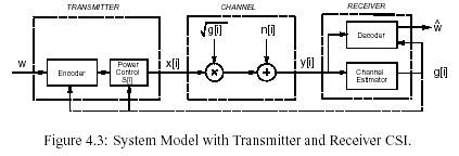
When both the transmitter and receiver have CSI, the transmitter can adapt its transmission strategy relative to this CSI, as shown in Figure. In this case there is no notion of capacity versus outage where the transmitter sends bits that cannot be decoded, since the transmitter knows the channel and thus will not send bits unless they can be decoded correctly. |
|
|
|
 |
|
|
|
 |
|
|
|
3. Capacity of Frequency Selective Fading Channels |
|
|
|
In this section we consider the Shannon capacity of frequency-selective fading channels. We first consider the capacity of a time-invariant frequency-selective fading channel. This capacity analysis is similar to that of a flat fading channel with the time axis replaced by the frequency axis. Next we discuss the capacity of time-varying frequency-selective fading channels. |
|
|
|
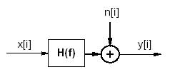
3.1 Time-Invariant Channels |
|
|
|
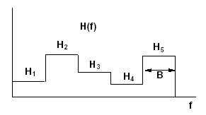
Consider a time-invariant channel with frequency response H(f), Assume a total transmit power constraint P. When the channel is time-invariant it is typically assumed that H(f) is known at both the transmitter and receiver. |
|
|
|
 |
|
|
|
Time-Invariant Frequency-Selective Fading Channels |
|
|
|
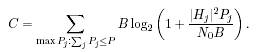
Let us first assume that H(f) is block-fading, so that frequency is divided into sub channels of bandwidth B, where H(f) = Hjis constant over each block, The frequency-selective fading channel thus consists of a set of AWGN channels in parallel with SNR : |
|
|
|
 |
|
|
|
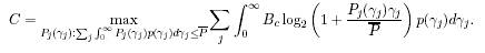
where Pj is the power allocated to the jth channel in this parallel set. The capacity of this parallel set of channels is the sum of rates associated with each channel with power optimally allocated over all channels. |
|
|
|
 |
|
|
|
Note that this is similar to the capacity and optimal power allocation for a flat-fading channel, with power and rate changing over frequency in a deterministic way rather than over time in a probabilistic way. |
|
|
|
 |
|
|
|
Block Frequency-Selective Fading |
|
|
|
3.2 Time-Varying Channels |
|
|
|
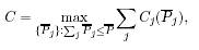
The time-varying frequency-selective fading channel is similar to the model shown. except that H(f) = H(f, i), i.e. the channel varies over both frequency and time. It is difficult to determine the capacity of time-varying frequency-selective fading channels, even when the instantaneous channel H(f, i) is known perfectly at the transmitter and receiver, due to the random effects of self-interference (ISI). |
|
|
|
We can approximate channel capacity in time-varying frequency-selective fading by taking the channel bandwidth B of interest and divide it up into sub channels the size of the channel coherence bandwidth Bc. We then assume that each of the resulting sub channels is independent, time-varying, and flat-fading with H(f, i) = Hj [i] on the jth sub channel. Since the channels are independent, the total channel capacity is just equal to the sum of capacities on the individual narrowband flat fading channels subject to the total average power constraint, averaged over both time and frequency: |
|
|
|
 |
|
|
|
where Cj(Pj) is the capacity of the flat-fading sub channel with average power P j. |
|
|
|
 |
|
|
|
Channel Division in Frequency-Selective Fading |
|
|
|
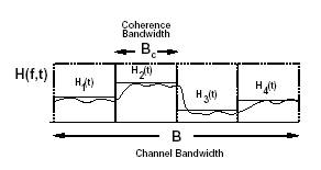
The Shannon capacity with perfect transmitter and receiver CSI is given by optimizing power adaptation relative to both time (represented by gj [i]= gj )and frequency (represented by the sub channel indexj) : |
|
|
|
 |
|
|
|
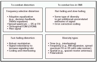
4. Mitigation to Combat Frequency-Selective Distortion |
|
|
|
Spread-spectrum techniques can be used to mitigate frequency- selective ISI distortion because the hallmark of any spread-spectrum system is its capability to reject interference, and ISI is a type of interference. Consider a direct sequence spread-spectrum (DS/SS) binary phase shift keying (PSK) communication channel comprising one direct path and one reflected path. The use of DS/SS is a good way to mitigate such distortion because the wideband SS signal would span many lobes of the selectively faded frequency response. Hence, a great deal of pulse energy would then be passed by the scatterer medium. |
|
|
|
Frequency-hopping spread spectrum (FH/SS) can be used to mitigate the distortion due to frequency-selective fading, provided the hopping rate is at least equal to the symbol rate. Compared to DS/SS, mitigation takes place through a different mechanism. FH receivers avoid multipath losses by rapid changes in the transmitter frequency band, thus avoiding the interference by changing the receiver band position before the arrival of the multipath signal. |
|
|
|
 |
|
|
|
Basic mitigation types |
|
|
References |
|
|
|
|
|
|
1. Andrea Goldsmith ?Wireless Communications?, Cambridge University Press, 2005. |
|
|
|
2. B. P. Lathi ?Modern Digital and Analog Communication Systems?, Oxford University Press, 1998. |
|
|
|
3. Behrouz A. Forouzan ?Data Communications and Networking?, Mc Graw Hill, 2002. |
|
|
|
4. IEEE Magazine, July 1997, pages from 102 to 109. |
|