According to the eigenvalues, it appears four or five
principal components should be used for the analysis.The first four
eigenvalues were all greater than one.The fifth eigenvalue was close to one, but it
does not explain more of the variability than any one individual variable would
(1/17 � 0.0588).76.85% of the variability is explained by the first four principal
components, and 82.41% of the variability is explained by the first five
principal components.The scree plots also suggest we should use the first four principal
components.The plot starts to slightly level off at the fifth principal
component.
Principal Components
Prin1
Prin2
Prin3
Prin4
Sports
0.034248
0.442066
-.089001
-.271723
SUV
0.129805
-.224212
-.493642
-.152413
Wagon
-.031771
-.019550
-.028867
0.862708
Minivan
0.053535
-.207014
0.276028
-.341532
AWD
0.092776
-.143740
-.551073
0.080692
RWD
0.117336
0.374878
0.243227
0.075547
SRP
0.258893
0.345468
-.016672
0.046504
DealerCost
0.257356
0.346102
-.014498
0.051591
Engine
0.339550
0.002649
0.048765
-.001305
Cylinders
0.326164
0.079670
0.065943
0.056018
Hp
0.311395
0.234928
-.004498
0.018717
Cmpg
-.306206
0.017018
0.141743
0.004267
Hwympg
-.306161
0.043666
0.247651
0.026109
Weight
0.331723
-.182569
-.085671
0.014675
WheelBase
0.254688
-.306301
0.284592
0.057582
Length
0.240991
-.269975
0.335648
0.099536
Width
0.288698
-.216703
0.137418
-.085770
When looking at the first four
principal components, we noticed some interesting
patterns.
Principal
Component #1:This principal component appears to be a contrast between Cmpg, and
Hwympg versus SUV, AWD, RWD, SRP, DealerCost, Engine, Cylinders, Hp, Weight,
WheelBase, Length, and Width.It almost seems to be comparing vehicles with
high and low gas mileages.For instance, vehicles that get lower gas
mileages tend to have larger engines, more horsepower and cylinders, and bigger
weights and sizes.Therefore, this principal component might be suggesting that vehicles
with higher city and highway gas mileages will have lower principal component 1
scores, whereas vehicles with lower city and highway gas mileages may have
higher principal component 1 scores.
Principal Component #2:This principal
component appears to be a contrast between Sports, RWD, SRP, DealerCost,
Cylinders, and Hp versus SUV, Minivan, AWD, Weight, WheelBase, Length, and
Width. Overall, it seems to be a contrast between
Sports cars and other vehicles.This is because sports cars tend to have
higher SRPs and Dealer costs, more Horsepower, and are RWD, which all cause the
principal component 2 scores to increase.
Principal Component #3: This
principal component appears to be a contrast between Sports, SUV, AWD, and
Weight versus Minivan, RWD, Cylinders, Cmpg, Hwympg, WheelBase, Length, and
Width. This could possibly be interpreted as a
contrast between minivans and SUVs.
Principal Component #4: This
principal component appears to be a contrast between Sports, SUV, Minivan, and
Width versus Wagon, AWD, RWD, and Length. A more simple explanation of the
contrast in this case could be that it is a contrast between Wagon and the other
vehicle types.
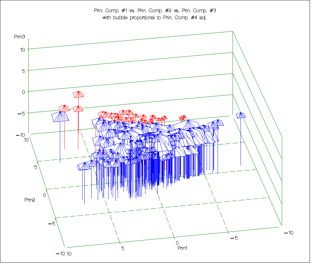
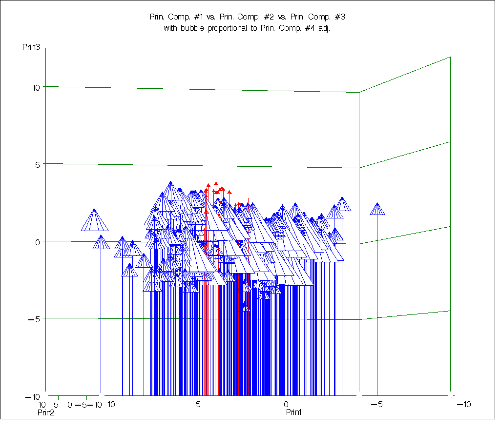
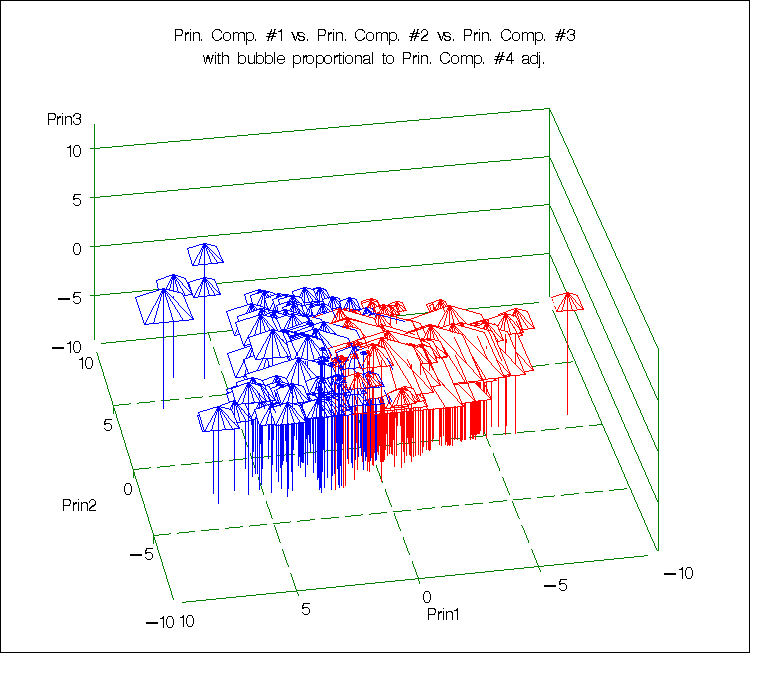
Let's check out some plots to help visualize these
patterns....
Plots
Red = Sports Cars Blue = Other
Vehicles
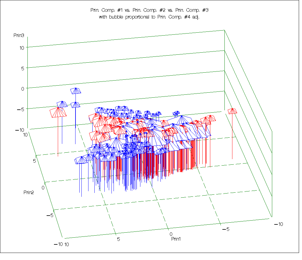
Red = Cars Blue = Other
Vehicles
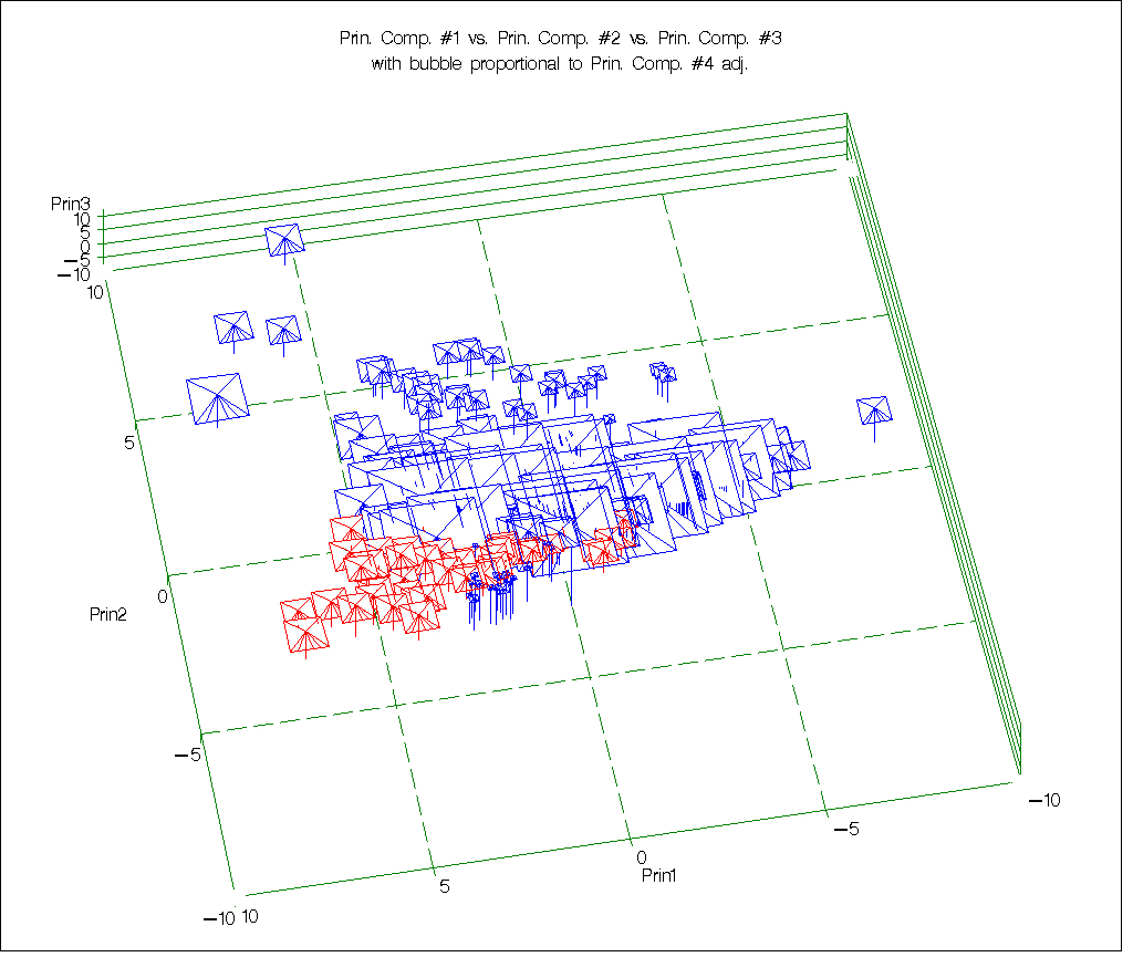
Red = SUVs Blue = Other
Vehicles
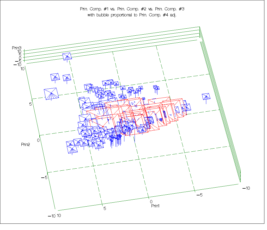
Red = Wagons Blue = Other
Vehicles
Red = Minivans Blue = Other
Vehicles
Red = Cmpg >=19
(median) Blue = Cmpg < 19
(median)