Matching Graphs Using the Pasco Interface

Abstract:

By determining how the sonic ranger can be used to produce different graphs, a set of distance versus time graphs and one of velocity versus time graphs were created. The graphs were then converted to the other type (i.e. distance versus time was converted to velocity versus time) in order to deduce the relationship between distance/time and velocity.

  *        *        *

                This was lab designed to use the sonic ranger and Pasco interface to recreate graphs of distance versus time, and velocity versus time. There were four graphs given, plus one bonus graph. Two of these graphs were distance versus time graphs, and the other two were velocity versus time. The bonus was velocity versus time.

                The first step in this lab was familiarizing ourselves with the sonic ranger. After we knew how the program worked and what motion would generate which results, we began the work of recreating the given graphs. Graph I[1]:

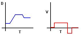
The graph on the left is the graph we were given. We recreated this graph by holding the object (a large cardboard box attached to a skateboard) steady, then pulling it back quickly and holding it steady there, then pushing it quickly for a shorter period of time than the first motion, then holding it steady for the remaining time.

After we had created this distance versus time graph, we needed to create a graph showing the relationship between velocity and time for the same motion. By using the following pair of graphs that were shown to us by our skilled instructor as an example of how to convert a distance versus time graph to a velocity versus time graph, we were able to analyze the action and convert it to the velocity versus time graph:

In our distance versus time graph, the object is not moving, then moves away steadily from the target. It moves closer for a shorter period of time, then stays still for the remainder of the test period. Our velocity versus time graph shows the object with no velocity (velocity is the change in distance divided by the change in time, so if the change in distance is zero, the velocity must be zero as well), then with a positive velocity. Since the object stops at this point in time, the velocity stops as well. When the object returns to motion, it has similar movement as the first movement, but this time, the velocity is negative because the object is becoming closer to the sonic ranger. Finally, the velocity versus time graph rounds out itself with a straight line at zero velocity for the period during which it was at rest.

 Graph II: 

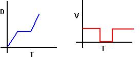
This is another distance versus time graph. In this graph, the distance steadily increases for a short period of time, suddenly decreases at the same velocity for a shorter period of time, then increases for the short period of time at the same velocity. Using the same skateboard-cardboard box apparatus, we pulled the board away from the sonic ranger slowly, then pushed it in at a slightly faster rate, then pulled it away again at the first pace.

The velocity versus time graph shows a steady increasing (thus positive) velocity, then a negative velocity (decreasing because the object is moving towards the sonic ranger), then the same positive velocity.

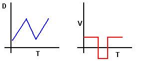
Graph III:

                This is the first velocity versus time graph. It shows a slow velocity, then a very rapidly decreasing one, then a slow negative velocity. To reproduce this graph, we pushed the apparatus slowly away from the sonic ranger, then pulled it back in the same direction faster so it was gaining speed, then pushed it forward quickly, stopped it suddenly, and let it rest for a few moments.

                Like as for the other graphs, the next step was to convert to the other ‘style’ of graph. In past cases, we converted distance versus time to velocity versus time. However, here we have a velocity versus time graph already, so we needed to convert this graph to distance versus time. Our handy instructor gave us an example of this process as well:

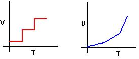
This shows a stable but low velocity, then a median stable velocity, then finally a high stable velocity. To show this as distance versus time, we needed to keep in mind the fact that velocity is simply distance divided by time. The corresponding graph of distance versus time of this sample motion shows the slow velocity (a slow increase in distance over the time), then the middle velocity (a medium increase in distance over the period of time), and lastly the high velocity, where a great distance was traveled in the same equal period of time.

                Our velocity versus time graph shows the slowly increasing velocity, which is the same as the first segment on the sample graph. The second segment shows a swift decrease from positive to negative distance, which accounts for the corresponding swift decrease in velocity (time cannot be decreasing in this situation, so the distance must be), and finally a negative distance which accounts for the negative velocity.

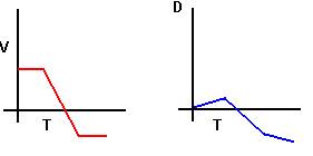
Graph IV:

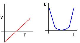
                The given graph shows a steadily increasing velocity, beginning at a negative position and rising to a positive position. To obtain this graph, we had to start the skateboard at a certain position to create a zero point, then move it closer in to bring the line to a negative velocity, then pull it away slowly at the same time it was brought towards the ranger.

                The velocity versus time graph of a steadily increasing velocity was then used to produce a distance versus time graph of the same motion. Because the initial velocity is negative, the distance from the object to the ranger in relation to the zero point is increasing, hence the downward slant of the line. The object then reaches the zero point, and enters positive velocity, and thus positive distance, as it moves away from the zero point and the ranger.

BONUS Graph:

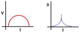
                This graph of velocity versus time shows increasing velocity, but it is not 100% steady. Instead, it goes up quickly and slowly slows down until it stops and heads downward. This motion is like that of any projectile object, which will travel in the pathway of a parabola when thrown. To recreate this graph, the cart with the box on it was pulled back quickly and the velocity slowed down until it reached nothing, then slowly headed back toward the ranger at the fast rate and decreased slowly.

                The conversion of the velocity versus time graph to that of distance versus time shows each separate distance, with some closer to the zero point and then getting farther away, and ultimately reaching a peak and returning to the zero point.

                After we figured out how to manipulate the Pasco interface apparatus to create the lines/graphs we wanted, the only problem we encountered in trying to produce the separate graphs were that two of our graphs (which were quite precise) had to be redone because they didn’t contain enough points. These were redone to achieve the same picture.