Version 1B:
September 27, 2004
Mars Forum “blueberry” measurement project
final report
Henry C. Wallace [email protected] (the author to which
correspondence should be sent.)
Abstract: An Internet collaboration via the Mars Forum
http://www.markcarey.com/mars/mars-forum/forum.html
has resulted in the Martian “blueberries” being
studied. As of this writing, 96 images have been studied from photographs taken
by the microscopic imaging camera carried by the NASA/JPL Opportunity rover.
From these images 245 spherules were evaluated and measured. For various
reasons 41 measured spherules were eliminated. The remaining 204 spherules have
been graphed and a “best fit” to the data obtained. It has been determined that
the data is most simply represented by a Weibull distribution function. This
distribution is highly suggestive of the “logistic growth model” familiar to
biologists, rather than the “lognormal” distribution familiar to geologists and
typical of concretions. It is suggested that a similar Devonian era land plant,
Pachytheca Hooker, might be related to the Martian blueberry. Confirmation of
the discovered statistics is shown from other Mars images, using automated
measurements.
Background
When NASA successfully landed
the Jet Propulsion Laboratory’s Opportunity rover on Mars, on a geologic
mission, they began to post .jpg images on the Internet at http://marsrovers.jpl.nasa.gov/gallery/all/
A discussion group formed up to discuss
the mission and these photographs at the Mars Forum. An immediate source of
interest was in what NASA/JPL begin calling “blueberries”. These are generally
small, almost spherical objects littering the Martian surface.
It was soon recognized that the
spherules had certain consistencies in color, shape and size. And it was
understood that, using the microscopic imaging camera (MI), these spherules
could be recognized and counted. A thread, “Go Measure…” was started on the
Open Mars Forum to solicit aid in the counting task.
Methods
The MI is one of the three cameras
carried by Opportunity, and takes closeup photographs of a small area of the
Martian surface which is only 1.2 inches by 1.2 inches (30.7 millimeters by
30.7 millimeters). In the camera this image is divided into 1024 by 1024
pixels. Thus a properly focused image can be used to fairly accurately measure
distance on the Martian surface: 1024 pixels divided by 30.7 mm is 33.36 pixels/mm,
or 0.03 mm/pixel. Thus a spherule having a maximum major diameter of 100 pixels
is understood to have a maximum major diameter of 3.0 mm.
Measurements were taken of the maximum
major diameter of each spherule. When this diameter was either horizontal or
vertical the pixels were read directly from the monitor screen. If the maximum
diameter laid across the spherule at an angle, the sum of the squares of the
vertical pixels and the horizontal pixels was determined and its square root
taken to determine the measurement.
A conservative set of rules was
developed by R. Lewis to assure consistent and proper “collecting” of the data. There
has been considerable cross checking of the results, and elimination of some of
the counted spherules during these cross checks. The result is that the useable
spherule count currently stands at 204. Forty-one (41) spherules have been
eliminated, mostly because they were considered to be “partial”. This means
that they were broken berries, or only partially exposed.
From the outset, it was understood that
only spherules above a certain diameter could be accurately tabulated. The MI
is limited it its magnification, and distinguishing a spherule from sand grains
or small spherical rocks limits its applicability to spherules greater than
about 1.2 mm in diameter. The collected data reflects this, and the results
obtained appear reasonable.
Data
The current list of raw data, and the
conservative rules of spherule collection, is being maintained by R. Lewis, at his site
http://geocities.com/rlewis6/Spherule_Database.htm
The list of data, as of this writing,
is attached at the end of this report.
One objective which emerged early in
this project was to properly graph and, as far as possible, characterize the
data. The best graph of the data is to generate a histogram from it. A
histogram divides the data into an undetermined number of “bins”, each
containing a certain constant range
of spherule sizes. The horizontal axis of the histogram is the average size of
the spherules in the bin, and the vertical axis is the number of spherules
contained in each bin. The range of spherule diameters contained in each bin,
as well as the location of each bin, has been a source of much consideration.
An
unexpected result from our data was the “tightness” with which the spherules
clustered around 4.19 mm. We had expected the distribution to be a standard
Gaussian, offset by 4.19 mm. Another unexpected result was the “hard limit” of
size distributions at the high end. The expected value of the current data (N=204) was
discovered to be 3.89 mm, and the standard deviation was discovered to be 0.86
mm. The Central Limit Theorem implies
that the expected value of the general population of Mars blueberries is within
7.0% of the 3.89 mm expected value of our 204 samples.
No spherules were discovered above about 5.7 mm, only 1.76 standard deviations above our data peak.
A Weibull population was suggested by
James Nelson. The Weibull has the characteristics of tightness and being
size-limited from above. Being a “recognized” statistical distribution was also
helpful. So the project was initiated of trying to find a best fit between our
collected data and a Weibull population. Or perhaps even between our data and
the sum of a major Weibull and a minor Weibull, if a second population became
evident. R. Lewis was the first to suggest the possibility of two or more berry
populations within our collected data, and this has not been ruled out as a possibility.
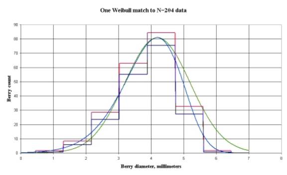
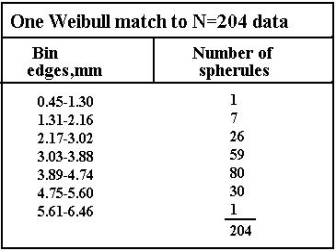
In the Table is shown the data used to
generate the histogram of the one Weibull match to the data. In this figure the
blue line represents the Weibull, the red histogram represents the positive
statistical error n+1/2sqr(n), and the black histogram represents the minus
statistical error n-1/2sqr(n). The green line is the standard Gaussian. The
bins are each 0.86 mm, or one standard deviation. Although the Weibull matches
the data almost exactly, and with more care could be brought into a perfect
match, the standard Gaussian does not miss by much.
The equations for the Weibull are shown
here:
http://www.systat.com/products/TableCurve2D/help/?sec=1247
The Weibull is designated by four
constants, a, b, c, and d. It is also a function of x. The constant a is the
amplitude of the Weibull at its peak. The constant b is the x-location of the
peak value. The last two constants, c and d, are “matching” constants used for
fitting the Weibull to the histogram. The constants used were a=81.0, b=4.19,
c=6.50, d=8.00.
Error Analysis
Throughout the data collection process,
we have been conscious of two possibly avoidable sources of potential error.
These are “focus errors” from the MI camera, and “human error”, principally
from interpreting the pixel edges in the MI images. This ignores the other
human errors such as transcription errors, etc., which we think we have
eliminated by our cross checking. The largest of these two sources of possible
errors is the focus error, and the human error has been absorbed into the focus
error.
Poorly focused MI images were not used.
By comparing MI images made at different times but of the same subjects, it was
determined that, even in apparently well focused images, a error of about 10%
existed. This has been attributed to the MI being either closer or further from
the subject. When multiple images were available, the better focused image was
used. This was not always possible, however.
The largest error, however, is the
statistical error resulting from the limited number of samples contained in any
one bin of the histogram. In any one bin, this RMS error is approximately the
square root of the number of spherules in that bin. The limits on the errors
are shown on the Figure “One Weibull Match” and on the corresponding Table.
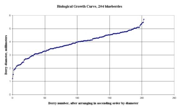
Biological Growth Curve
The simplest meaningful
display of the raw, collected data is to first arrange the data into a list by
increasing berry diameter, then to plot these increasing diameters as the
vertical axis, with the berry number as the horizontal axis. The result is
called the “Biological Growth Curve”. Although not definitive, we think there
is a clear implication that the Mars blueberries are the result of organic
growth.
The following thought
experiment illustrates a procedure by which biologists extract growth data from
living populations. See, for instance,
http://www.findarticles.com/p/articles/mi_m0FDG/is_3_101/ai_107524533/pg_3
http://www.id.unizh.ch/software/unix/statmath/sas/sasdoc/stat/chap46/sect6.htm
http://fishbull.noaa.gov/994/loh.pdf
http://www.worldfishcenter.org/Naga/naga26-4/pdf/naga-26-4-article2.pdf
http://www.stat.nus.edu.sg/~wangyg/Research/pub/MS030919.pdf
A catfish farmer wanted to know how many millimeters per day his
catfish grew. He could have started with an empty pond, and put in 10,000
fingerlings. Then each following day he could have measured a few, and recorded
their average length. A graph with days along the bottom and length along the
side would have then been his “fish growth curve”.
But he didn’t want to lose the production of a perfectly good pond
for all those days. He also had a pond which was in continuous use, into which
he would put 10,000 new fingerlings every day. He had a catching system
installed, which would remove the mature fish continuously when they reached
market size. It was an efficient system: each day he would recover 10,000 big
fish ready for market, to replace the 10,000 fingerlings he added each day.
It took 100 days for a fish to reach market size, so this pond
contained 1,000,000 fish on the average day. One day he took out 10,000 fish
for a test. Because this was a random sample, every size fish was in the
sample. Every age fish was equally represented in this sample, so it contained
about 1% fingerlings, 1% one-day old fish, 1% two day old fish, and so on up to
1% mature fish. One percent of the 10,000 fish sample is 100 fish, so he had,
in his sample, 100 fingerlings, 100 one day old fish, and so on up to include
one hundred mature fish.
He measured the length of each fish, then arranged the lengths on
a list by increasing length. He assumed that each longer fish represented an
older fish. He took the 100 shortest fish, the fingerlings, and averaged their
length and figured that length represented a one day old fish. He took the next
100 fish, averaged their length, and figured that represented a two day old
fish. So on, up to get the length of every age fish in the sample. He now had
100 measurements, each representing the length of the fish one day older, for a
total of 100 days.
He made a graph, with the 100 days across the bottom, and the
measurements up the left side. He had his “fish growth curve”, without losing
the 100 days production from a perfectly good pond.
This illustrates how
statistical sampling is used to draw growth data from a living population. It
is also obvious that if the population were quickly frozen in time and
preserved, the same statistical sampling could still be used to determine the
prior growth characteristics of the now deceased population.
Because we have performed
exactly the same operation, that is, collecting a random sample of the Martian
blueberry population, we suggest the “Biological Growth Curve” has meaning
within the limits of the small number of samples thus far taken. Our intention
is to continue the collection effort, and to eventually include in our sample
every available blueberry from every MI image.
Note the growth curve
begins with a period of high growth rate up to berry diameters of about 3.8 mm.
It then goes through a region of almost linear growth up to a berry diameter of
about 5.1 mm, and terminates in another rapid growth region up to the maximum
berry diameter of 5.7 mm. The sudden, smooth upturn in growth rate above about
5 mm was entirely unexpected. It has, however been replicated by other means:
see the section “Confirmation
from automated data collection”. We have no
explanation for this “late growth spurt”, and it is a phenomena for which we
solicit comments from biologists. This late growth spurt is necessary,
apparently, for completion of the upper right portion of the logistic sigmoid
(or S-shaped) curve.
For the case of the
Martian blueberries, the horizontal axis has the intrinsic dimension of time,
but the units of time are not presently known. To date the authors have seen no
rover photographs showing sufficient changes with time to establish the time
units. Indeed, many support the theory that the blueberries are a fossilized
population. It is hoped that time-lapse MI photography might be applied by
NASA/JPL to perhaps settle this question. Indications are that lapses of two
days do not indicate growth, so
longer lapses will probably be required. If this is undertaken, the blueberries
will likely show most growth when in the size ranges of 1-3 mm or 5-5.7 mm.
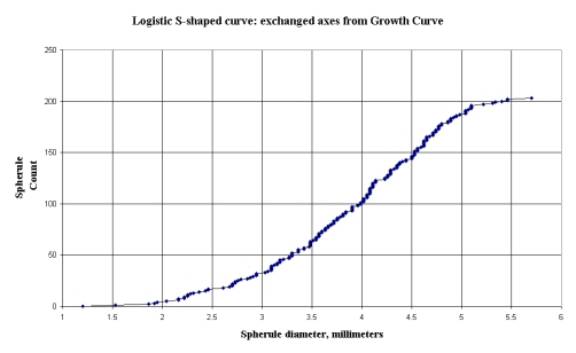
By simply exchanging the
horizontal and vertical axes of the growth curve, the S-shaped curve is
generated.
The “tightness” with which
the blueberry population is clustered is difficult to describe verbally, so two
illustrations will be presented. The largest blueberry is 5.7 mm in diameter,
and the most common are 4.19 mm in diameter. The largest berry’s diameter is
about the thickness of three nickels sandwiched together, and the most common
about like two nickels. The bottom of the S-shaped curve breaks at a berry
diameter of 3.8 mm (like three dimes), and the top breaks at 5.1 mm (like four
dimes). Yet between these two dimensions, an increase of only 32% in berry
diameter, is the “linear growth region” of the berry population.
Another illustration of the
tight grouping exhibited by the blueberries, and one which will be recognized
by many readers, comes from “sieving” the blueberry population:
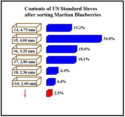
Compare this distribution to that of
the "Moqui
Marbles", the concretions which have been mentioned as a likely candidate
for an Earthly analog to the Mars blueberries. All
blueberries are much smaller than the smallest of the “Moqui Marbles” shown at
the following four sites:
http://www.utah.edu/unews/releases/04/jun/marsmarbles.html
http://www.nature.com/cgi-taf/DynaPage.taf?file=/nature/journal/v429/n6993/full/429707a_fs.html
http://deseretnews.com/dn/view/0,1249,595071060,00.html
http://www.spaceflightnow.com/news/n0406/16blueberries/
These concretions, because of the wide
fifty to one variability of sizes shown, appear to follow a lognormal
population distribution. Most geological structures, such as natural crystals
and ores (See Geological References), exhibit such wide ranges of sizes, from
sand to boulders. The population
densities of these is commonly represented by a lognormal or another of the
“extreme value” distribution, which is characterized by a peak followed by a
“tail” to the right. The tail into ever
increasing sizes admits to no “upper size limit”.
The blueberries, on the other hand,
closely follow the “logistic growth model” familiar to biologists (See
Biological References). The relationship between the Weibull distribution and
the logistic distribution is now well established. The logistic, Weibull,
Richards, Gompertz and other
growth functions are now used almost interchangeably by biologists, and growth
functions is a subject of current interest among mathematical biologists.
See, for instance
http://aob.oupjournals.org/cgi/content/full/91/3/361
and
http://www.udl.es/usuaris/q3695988/WebPL/PagGene/PagTuto/T1/T1_4/Canonical%20representations.700.htm
An additional growth function is used
almost exclusively by fishery biologists, and is called the von Bertalanffy growth function (vBGF).
Fish populations typically follow a Gaussian population distribution, while
their growth is usually parametized using the vBGF.
The logistic population distribution
is characterized by a tail to the left terminated on the right by a hard
limited upper peak. The hard limit on
larger sizes allows no members of the population above a certain size. The
hard limit in diameter is indicative of an organism which has run into a limit
of resources.
Percent composition of hematite
Suggestions have been made
that the blueberries are composed of hematite (Iron III). The instruments
carried by the Mars rovers which might make such a determination are the Alpha
Particle X-Ray Spectrometer (APXS) and the Mossbauer Spectrometer. The
specifications of these spectrometers are at
http://athena.cornell.edu/pdf/tb_apxs.pdf
and at
http://athena.cornell.edu/pdf/tb_moss.pdf
These are both
surface-reading devices. They can only make iron measurements to a maximum
depth of 100 micrometers (APXS) and an average depth of 300 micrometers
(Mossbauer) into the surface at which they are directed.
The total volume of a 4 mm
diameter sphere is 16.76 cubic millimeters. The volume of its outer shell, if
of thickness 300 micrometers (0.3 mm), is
4.65 cubic millimeters. If the entire outer shell were composed of hematite,
the percent by volume this shell would represent is 28%. Thus 28% by volume is
the maximum hematite composition which the Mars rovers can certify.
Neither of these
spectrometers can look inside this outer shell, to make determination of the
materials composing the other 72% of the blueberry. The remaining 72% of the
berry volume might, for instance, be high in the carbon indicative of past or
present life.
It is likely that NASA/JPJ
would be more comfortable with hematite measurements made by the APXS, which is
optimized for iron measurements but has a maximum measurement depth of 0.1 mm.
In this case, the shell thickness would be 0.1 mm, and would comprise 9.7% of
the volume of the sphere, leaving the other 90.3% of the sphere of undetermined
materials.
The question of Volcanic origin:
Lapilli
Volcanic lapilli have been suggested
as a possible explanation for the Martian blueberries. This suggestion is
implausible because of the sheer number of the berries, their striking
similarities, and by their apparently wide geographical dispersal. But the
strongest argument against lapilli is again the tight dimensional constraints
and the statistics of the berry population.
Lapilli is but a name given to a range
of “tephra” emitted volcanically. By its very nature, tephra has a lognormal or
other “extreme value” distribution, because there are vastly more sand grains
emitted by a volcano than there are boulders. Because lapilli is but a
“section” of this tephra population, it, too, would be expected to have a
lognormal distribution.
http://vulcan.wr.usgs.gov/Glossary/Tephra/description_tephra.html
Confirmation from automated
data collection
Denis Royer [email protected] has been collecting
data from Panoramic Camera images using pattern recognition software. The
Panoramic Camera (pancam) is also carried by
both Mars rovers, but is not a closeup camera like the MI. His work is
documented at his site
http://perso.club-internet.fr/droyer/mars/mars1_000001.htm
and generally confirms the
statistics reported here. The strength of this technique of data collection is
the number of blueberries which can be captured in a single pancam image: in a
single Mars Sol day 202 pancam image,
he collected 1,875 spherules purported to be blueberries! The weakness of this
technique is the inherent inaccuracy of using the lower resolution images from
the pancam, and of turning the selection and measurement of the blueberries
over to a computer program. There is also a “noise” term in the computer
generated data which must be subtracted out to provide accuracy, particularly
for small berry diameters. As of this writing, D. Royer reports difficulty in
measuring berry diameters less than about 1.75 mm.
Using data from D. Royer, the
following growth curve was generated from the Sol 202 pancam data:
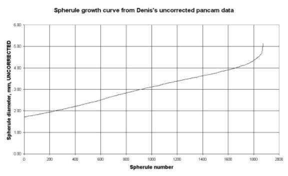
You will notice the upturn in
growth rate for larger spherules, and the long linear growth, which confirms
the MI data reported elsewhere in this report. This figure uses uncorrected
data. There is certainly some sort of correction which could be made, to
“calibrate” the automated data collection with the MI data collection. For instance,
the peak of the Weibull matching the Sol 202 data could be caused to occur at
4.19 mm as it does for the MI data. Or the largest berry could be caused to be
5.7 mm as for the MI data. However, the automated pattern recognition software
uses “filters” which affect different berry diameters in different ways. This
nonlinear treatment by the software seems to occlude any simple multiplicative
correction.
The case for Pachytheca Hooker
http://www.xs4all.nl/~steurh/engpach/epachy.html
During the lower Devonian
times, one of the first Earthly experiments in land plants was the now
fossilized Pachytheca Hooker. While
this plant carried its own water resources, thus could survive on land, it had
not developed the leaves now associated with land plants. Like the Martian
blueberries, it was a spherical plant of 1-6 mm diameter. It is thought that Pachytheca was capable of
photosynthesis. It was an extremely simple plant, little more than a colony of
single celled organisms similar to algae.
Being a plant, there is every reason to think that the population
density of Pachytheca Hooker will
obey the logistic growth model, although we are not aware of any measurements
from the fossil record which would support or refute this.
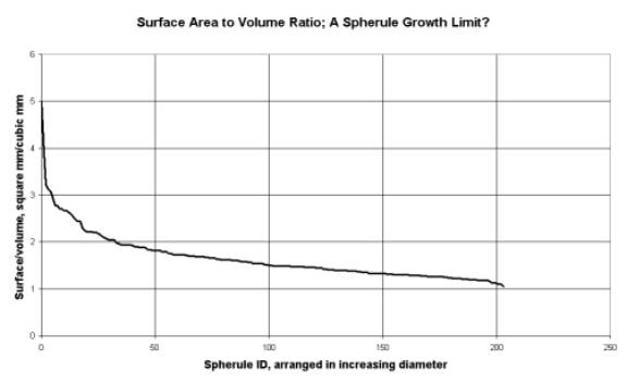
Not having leaves, the
light-collecting surface of Pachytheca was limited to its outer
spherical surface. Because the surface of the spheres increases as the square
of the diameter and the volume of the spheres increases as the cube of the
diameter, a spherical plant is limited in the diameter to which it can grow. As
its diameter increases, a spherical plant reaches a point at which the light
collected on its outer surface can no longer support the living population of
cells within the sphere. This is an example of resource-limited growth (See Pachytheca Hooker references).
Although not the only
possible explanation of resource limitation on the Mars blueberry growth, the
following figure of blueberry surface/volume vs. berry diameter might possibly
argue for a photosynthesis limit. From this figure, it might appear that the
berries “run out of sunlight” at a Volume/Surface just over 1mm.
Credits:
James Nelson, [email protected]
R. Lewis, [email protected]
The author would also like to thank
Richard Baumeister and Mark Carey for moderating and providing the Mars Forum,
and the many workers a NASA/JPL for providing the images without which this
work would not have been possible. We would like to thank Ian Lyon [email protected] for his help with
statistical error analysis. We also owe a debt of gratitude to the many
wonderful participants on the Forum, for their many supportive comments. We
also wish to thank, in particular, the several unnamed participants who aided
in the (ongoing) collection of the spherule data.
Biological references
http://www.langara.bc.ca/biology/mario/Biol1116notes/biol1216chap35.html
Good discussion of
exponential growth and logistic model, ecology.
http://www.emc.maricopa.edu/faculty/farabee/BIOBK/BioBookpopecol.html
Nice pictures, ecology.
http://www.tnstate.edu/ganter/B412%20Extra%20LogisticGrowth.html
Fair discussion.
http://www.geom.uiuc.edu/education/calc-init/population/logistic.html
Worked problems. Invasion of
pines.
http://www.aciar.gov.au/web.nsf/doc/JFRN-5J4725/$file/PR102%20Chapter%2016.pdf
Water hyacinths vs. weevils.
http://www.maa.org/reviews/mathbiomodels.html
Book review of mathematical
modeling in biology.
http://www.cnr.uidaho.edu/wlf448/comp1.htm
Geological references
http://www.bwk.kuleuven.ac.be/bwk/sr99/nar.htm#nr2.1
Diamonds, some ores.
http://www.minsocam.org/MSA/AmMin/TOC/Articles_Free/2002/Eberl_p1235-1241_02.pdf
Good reference.
http://www.dggs.dnr.state.ak.us/scan1/gr/text/GR48.PDF
Rocks and mining.
http://www.beg.utexas.edu/staffinfo/pdf/duttonAAPG2002.pdf
Calcite cement distribution…
http://dust.ess.uci.edu/facts/psd/psd.pdf
Ice crystals, good lognormal
discussion, statistics discussion.
http://geoecosse.bizland.com/softwares/Tutorial_stats.htm
http://geoecosse.bizland.com/softwares/
Excel geological statistics
package.
http://www.bae.uky.edu/UK-ARC/downloads/Papers/papers/Karstsyp.pdf
http://quebec.hwr.arizona.edu/research/shanahan00-africa.pdf
Pachytheca Hooker References
http://scienceweek.com/2003/sc031121-2.htm
On the
evolution of plant leaves.
http://www.for.gov.bc.ca/hfd/pubs/Docs/Rr/RR09.pdf
Pine leaves.
Raw Data
ID
Sol Pixels mm X Y Image Notes
1000
010 119 3.57 954 128 1M129070954EFF0224P2933M2M1 dimple
1001 010 40 1.2 58 658 1M129070954EFF0224P2933M2M1 dimple
1400 014 130 3.9 686 163 1M129426319EFF0300P2932M1M1
1401 014 . 113 225 1M129426319EFF0300P2932M1M1 partial
1402 014 125 3.75 955 539 1M129426319EFF0300P2932M1M1 seam
1403 014 160 4.8 771 831 1M129426319EFF0300P2932M1M1
1404 014 . 345 766 1M129426319EFF0300P2932M1M1 partial
1405 014 182 5.46 605 353 1M129426503EFF0300P2932M1M1
1406 014 170 5.1 121 400 1M129426503EFF0300P2932M1M1 seam
1407 014 . 615 489 1M129426503EFF0300P2932M1M1 partial
1408 014 . 436 593 1M129426503EFF0300P2932M1M1 partial
1409 014 150 4.5 661 689 1M129426503EFF0300P2932M1M1
1410 014 158 4.74 275 806 1M129426503EFF0300P2932M1M1
1411 014 65 1.95 938 916 1M129426503EFF0300P2932M1M1
1412 014 124 3.72 230 172 1M129430201EFF0300P2932M1M1
1413 014 116 3.48 494 532 1M129430201EFF0300P2932M1M1 seam
1500 015 174 5.22 843 564 1M129515786EFF0312P2933M2M1 seam in_situ
1700 017 64 1.92 604 579 1M129692504EFF0322P2953M2M1 dimple
1701 017 110 3.3 496 897 1M129692504EFF0322P2953M2M1 double
1702 017 81 2.43 438 918 1M129692504EFF0322P2953M2M1 double
1900 019 169 5.07 171 783 1M129869769EFF0338P2953M2M1
2500 025 . 470 356 1M130404446EFF0400P2953M2M1 partial dimple shiny
2501 025 . 260 372 1M130404446EFF0400P2953M2M1 partial shiny
2502 025 . 288 942 1M130404446EFF0400P2953M2M1 partial shiny
2503 025 . 474 778 1M130405277EFF0400P2953M2M1 partial
2504 025 . 380 898 1M130405277EFF0400P2953M2M1 partial
2600 026 . 460 370 1M130491519EFF0400P2953M2M1 partial
2800 028 . 630 70 1M130669714EFF0454P2953M2M1 partial in_situ rim
2801 028 . 104 828 1M130669714EFF0454P2953M2M1 partial in_situ rim
2802 028 136 4.08 320 338 1M130670237EFF0454P2953M2M1 in_situ
2803 028 128 3.84 958 114 1M130671782EFF0454P2953M2M1 in_situ rim
2804 028 112 3.36 920 834 1M130671782EFF0454P2953M2M1 in_situ rim
2805 028 116 3.48 356 292 1M130672582EFF0454P2933M2M1 double in_situ
2806 028 72 2.16 370 334 1M130672582EFF0454P2933M2M1 double in_situ
2807 028 . 946 882 1M130672582EFF0454P2933M2M1 partial in_situ
2808 028 114 3.42 590 530 1M130672935EFF0454P2933M2M1 seam in_situ
2809 028 . 426 878 1M130672935EFF0454P2933M2M1 partial in_situ
2900 029 . 120 394 1M130762321EFF0454P2953M2M1 partial in_situ
2901 029 138 4.14 502 596 1M130762321EFF0454P2953M2M1 in_situ
2902 029 . 752 598 1M130762321EFF0454P2953M2M1 partial in_situ
3400 034 . 821 242 1M131201618EFF0500P2933M2M1 partial shiny in_situ
3401 034 . 719 549 1M131201618EFF0500P2933M2M1 partial shiny in_situ
3900 039 126 3.78 771 186 1M131647757EFF0544P2951M2M1 in_situ
3901 039 . 864 600 1M131647757EFF0544P2951M2M1 partial in_situ
3902 039 153 4.59 105 462 1M131648183EFF0544P2951M2M1 in_situ
3903 039 112 3.36 351 30 1M131648609EFF0544P2951M2M1 in_situ
3904 039 143 4.29 453 78 1M131648609EFF0544P2951M2M1 in_situ petal?
3905 039 182 5.46 144 810 1M131648609EFF0544P2951M2M1 in_situ
3906 039 159 4.77 927 819 1M131649074EFF0544P2933M2M1 in_situ
3907 039 . 450 924 1M131649074EFF0544P2933M2M1 partial in_situ rim
3908 039 144 4.32 402 630 1M131649564EFF0544P2933M2M1 dimple in_situ
3909 039 74 2.22 311 355 1M131650610EFF0544P2933M2M1 in_situ
3910 039 155 4.65 210 171 1M131650751EFF0544P2931M2M1 in_situ
3911 039 110 3.3 228 459 1M131650751EFF0544P2931M2M1 in_situ
3912 039 145 4.35 213 666 1M131650751EFF0544P2931M2M1 in_situ
3913 039 . 483 594 1M131651465EFF0544P2933M2M1 partial in_situ
3914 039 146 4.38 75 675 1M131651465EFF0544P2933M2M1 in_situ
3915 039 98 2.94 618 696 1M131652949EFF0544P2933M2M1 in_situ
3916 039 . 363 132 1M131653435EFF0544P2971M2M1 partial in_situ
3917 039 . 564 159 1M131653435EFF0544P2971M2M1 partial in_situ
3918 039 . 771 759 1M131653435EFF0544P2971M2M1 partial in_situ
3919 039 . 84 96 1M131653947EFF0544P2972M2M1 partial in_situ
3920 039 168 5.04 210 537 1M131653947EFF0544P2972M2M1 in_situ
3921 039 142 4.26 522 855 1M131654125EFF0544P2972M2M1 in_situ
3922 039 143 4.29 285 303 1M131655288EFF0544P2971M2M1 seam shiny in_situ
3923 039 . 371 323 1M131655288EFF0544P2971M2M1 partial in_situ
3924 039 150 4.5 462 778 1M131655641EFF0544P2972M2M1 in_situ
3925 039 157 4.71 570 309 1M131656272EFF0544P2971M2M1 in_situ
3926 039 156 4.68 794 443 1M131656918EFF0544P2972M2M1 in_situ
3927 039 . 343 524 1M131656918EFF0544P2972M2M1 partial in_situ
3928 039 152 4.56 858 890 1M131656918EFF0544P2972M2M1 in_situ
4000 040 152 4.56 642 786 1M131733971EFF0544P2933M2M1 in_situ
4001 040 159 4.77 363 366 1M131734806EFF0544P2972M2M1 in_situ
4100 041 135 4.05 648 153 1M131830676EFF0574P2952M2M1 in_situ
4101 041 163 4.89 743 463 1M131832300EFF0574P2952M2M1 in_situ
4102 041 135 4.05 186 810 1M131832300EFF0574P2952M2M1 in_situ
4103 041 157 4.71 469 255 1M131833318EFF0574P2952M2M1 in_situ
4104 041 168 5.04 148 464 1M131834144EFF0574P2952M2M1 in_situ
4105 041 146 4.38 754 879 1M131834144EFF0574P2952M2M1 in_situ
4200 042 141 4.23 930 397 1M131912509EFF05A6P2951M2M1 in_situ
10500 105 118 3.54 297 75 1M137503553EFF2208P2956M2M1
10501 105 74 2.22 128 123 1M137503553EFF2208P2956M2M1
10502 105 105 3.15 57 179 1M137503553EFF2208P2956M2M1
10503 105 159 4.77 290 223 1M137503553EFF2208P2956M2M1
10504 105 93 2.79 901 97 1M137503553EFF2208P2956M2M1
10505 105 145 4.35 890 239 1M137503553EFF2208P2956M2M1
10506 105 89 2.67 110 551 1M137503553EFF2208P2956M2M1
10507 105 127 3.81 200 611 1M137503553EFF2208P2956M2M1 dimple
10508 105 124 3.72 468 600 1M137503553EFF2208P2956M2M1
10509 105 101 3.03 477 755 1M137503553EFF2208P2956M2M1
10510 105 123 3.69 920 559 1M137503553EFF2208P2956M2M1
10511 105 82 2.46 1002 672 1M137503553EFF2208P2956M2M1
10512 105 190 5.7 793 890 1M137503553EFF2208P2956M2M1
10600 106 121 3.63 172 141 1M137593003EFF2208P2956M2M1
10601 106 119 3.57 537 142 1M137593003EFF2208P2956M2M1
10602 106 87 2.61 668 220 1M137593003EFF2208P2956M2M1
10603 106 119 3.57 770 246 1M137593003EFF2208P2956M2M1
10604 106 116 3.48 871 338 1M137593003EFF2208P2956M2M1
10605 106 106 3.18 129 420 1M137593003EFF2208P2956M2M1
10606 106 104 3.12 132 419 1M137593003EFF2208P2956M2M1
10607 106 119 3.57 373 485 1M137593003EFF2208P2956M2M1
10608 106 118 3.54 290 578 1M137593003EFF2208P2956M2M1
10609 106 72 2.16 123 620 1M137593003EFF2208P2956M2M1
10610 106 91 2.73 882 595 1M137593003EFF2208P2956M2M1
10611 106 103 3.09 58 676 1M137593003EFF2208P2956M2M1
10612 106 62 1.86 173 787 1M137593003EFF2208P2956M2M1
10613 106 154 4.62 286 725 1M137593003EFF2208P2956M2M1
10614 106 137 4.11 876 737 1M137593003EFF2208P2956M2M1
10615 106 68 2.04 775 150 1M137593512EFF2208P2956M2M1 dimple
10616 106 114 3.42 100 186 1M137593860EFF2208P2956M2M1
10617 106 128 3.84 882 149 1M137593860EFF2208P2956M2M1
10618 106 103 3.09 554 425 1M137593860EFF2208P2956M2M1 in_situ
10619 106 136 4.08 930 377 1M137593860EFF2208P2956M2M1
10620 106 121 3.63 986 478 1M137593860EFF2208P2956M2M1
10621 106 77 2.31 943 617 1M137593860EFF2208P2956M2M1
10622 106 130 3.9 600 784 1M137593860EFF2208P2956M2M1 dimple
12200 122 95 2.85 199 737 1M139013191EFF2809P2956M2M1
12201 122 137 4.11 149 884 1M139013191EFF2809P2956M2M1
12400 124 . 299 983 1M139191289EFF2821P2956M2M1 partial in_situ, rim
12401 124 . 5 675 1M139191539EFF2821P2956M2M1 partial in_situ, rim
12402 124 . 114 913 1M139191539EFF2821P2956M2M1 partial in_situ, rim
12403 124 145 4.35 853 660 1M139191909EFF2821P2956M2M1 in_situ
12404 124 121 3.63 960 866 1M139191909EFF2821P2956M2M1 in_situ
12405 124 151 4.53 335 344 1M139192413EFF2821P2956M2M1 in_situ
12406 124 . 548 338 1M139192413EFF2821P2956M2M1 partial in_situ
12407 124 152 4.56 410 485 1M139192413EFF2821P2956M2M1 seam in_situ
12408 124 135 4.05 762 485 1M139192663EFF2821P2956M2M1 in_situ
12409 124 155 4.65 514 597 1M139192663EFF2821P2956M2M1 in_situ, rim
12410 124 137 4.11 1022 144 1M139194111EFF2821P2956M2M1 seam in_situ
12411 124 117 3.51 824 66 1M139194111EFF2821P2956M2M1 in_situ
12412 124 91 2.73 762 256 1M139194111EFF2821P2956M2M1 in_situ
12413 124 170 5.1 250 418 1M139194520EFF2821P2956M2M1 in_situ
12414 124 136 4.08 661 1019 1M139194520EFF2821P2956M2M1 in_situ
12415 124 141 4.23 147 747 1M139195771EFF2821P2956M2M1 seam in_situ
12500 125 92 2.76 432 236 1M139279994EFF2829P2956M2M1 in_situ
12501 125 107 3.21 822 120 1M139280490EFF2829P2956M2M1 in_situ
12502 125 98 2.94 428 729 1M139280691EFF2829P2976M2M1 in_situ
12503 125 115.6 3.47 178 232 1M139280874EFF2829P2956M2M1 in_situ
12504 125 110 3.3 412 194 1M139282897EFF2829P2956M2M1 in_situ
12505 125 150.8 4.52 470 95 1M139283222EFF2829P2956M2M1 in_situ
12506 125 154 4.62 787 850 1M139284464EFF2829P2956M2M1 in_situ
12507 125 145.4 4.36 445 822 1M139285367EFF2829P2976M2M1 in_situ
14200 142 . 886 154 1M140791929EFF3190P2957M2M1 partial
14201 142 147 4.41 794 260 1M140791929EFF3190P2957M2M1
14202 142 . 770 470 1M140791929EFF3190P2957M2M1 partial in_situ
14203 142 . 246 128 1M140792323EFF3190P2957M2M1 partial in_situ
14204 142 . 734 598 1M140792770EFF3190P2957M2M1 partial in_situ
14205 142 . 778 658 1M140793829EFF3190P2957M2M1 partial rim
14206 142 163 4.89 510 690 1M140794160EFF3190P2957M2M1 in_situ, rim
14400 144 . 26 858 1M140976080EFF3190P2956M2M1 partial in_situ
14401 144 137 4.11 615 453 1M140976080EFF3190P2956M2M1 in_situ
14402 144 134 4.02 926 330 1M140976080EFF3190P2956M2M1 in_situ
14403 144 148 4.44 422 216 1M140976352EFF3190P2916M2M1 in_situ
14404 144 138 4.14 154 896 1M140976567EFF3190P2916M2M1 in_situ
14405 144 . 512 748 1M140976687EFF3190P2916M2M1 partial in_situ
14406 144 143 4.29 723 720 1M140976848EFF3190P2906M2M1 partial in_situ, rim
14407 144 158 4.74 680 880 1M140977007EFF3190P2916M2M1 in_situ
14408 144 82 2.46 163 538 1M140977007EFF3190P2916M2M1 in_situ, irregular
14409 144 157 4.71 445 382 1M140977007EFF3190P2916M2M1 in_situ
14600 146 155 4.65 420 302 1M141149935EFF3190P2976M2M1 partial in_situ, rim
14601 146 170 5.1 272 859 1M141151027EFF3190P2977M2M1 in_situ
14800 148 137 4.11 789 781 1M141322163EFF3190P2977M2M1 in_situ, rim
15100 151 130 3.9 514 189 1M141588412EFF3200P2977M2M1 partial in_situ, rim
15200 152 177 5.31 66 720 1M141691232EFF3200P2907M2M1 partial in_situ, rim
15201 152 162 4.86 730 830 1M141691232EFF3200P2907M2M1 partial in_situ, rim
15800 158 120 3.6 302 436 1M142209459EFF3215P2957M2M1
15801 158 143 4.29 320 692 1M142209459EFF3215P2957M2M1
15802 158 112 3.36 805 767 1M142209459EFF3215P2957M2M1
16500 165 142 4.26 136 974 1M142829931EFF3221P2976M2M1
17400 174 151 4.53 215 64 1M143629781EFF3300P2977M2M1
17401 174 134 4.02 1023 889 1M143629781EFF3300P2977M2M1 double?
17402 174 154 4.62 739 940 1M143630076EFF3300P2977M2M1
17600 176 168 5.04 837 572 1M143807453EFF3328P2977M2M1 size scaled up 16% for
best focus
17601 176 122 3.66 888 582 1M143807771EFF3328P2977M2M1
17700 177 150 4.5 155 565 1M143896614EFF3336P2957M2M1
17701 177 118 3.54 609 385 1M143896614EFF3336P2957M2M1
17702 177 165 4.95 876 554 1M143896614EFF3336P2957M2M1
17703 177 170 5.1 320 939 1M143896614EFF3336P2957M2M1
17704 177 160 4.8 529 886 1M143896614EFF3336P2957M2M1
17705 177 168 5.04 946 852 1M143896614EFF3336P2957M2M1
17706 177 106 3.18 849 944 1M143896614EFF3336P2957M2M1
17700 177 136 4.08 885 485 1M143896909EFF3336P2957M2M1
17701 177 154 4.62 126 566 1M143896909EFF3336P2957M2M1
17702 177 90 2.7 779 558 1M143896909EFF3336P2957M2M1
17703 177 166 4.98 440 722 1M143896909EFF3336P2957M2M1
17704 177 158 4.74 228 745 1M143896909EFF3336P2957M2M1
17705 177 165 4.95 881 933 1M143896909EFF3336P2957M2M1
18100 181 154 4.62 926 840 1M144251471EFF3352P2977M2M1
18101 181 155 4.65 119 108 1M144251984EFF3352P2977M2M1
18200 182 154 4.62 550 246 1M144339348EFF3370P2957M2M1 double
18201 182 136 4.08 518 370 1M144339348EFF3370P2957M2M1 dimple double third
spherule?
18202 182 162 4.86 834 408 1M144339348EFF3370P2957M2M1
18203 182 105 3.15 240 425 1M144339348EFF3370P2957M2M1
18204 182 180 5.4 416 525 1M144339348EFF3370P2957M2M1
18205 182 . 268 526 1M144339348EFF3370P2957M2M1 partial
18206 182 164 4.92 786 649 1M144339348EFF3370P2957M2M1
18207 182 133 3.99 688 284 1M144339996EFF3370P2957M2M1 partial measurable
18208 182 122 3.66 880 337 1M144339996EFF3370P2957M2M1
18209 182 116 3.48 798 389 1M144339996EFF3370P2957M2M1
18210 182 143 4.29 237 886 1M144339996EFF3370P2957M2M1
18211 182 134 4.02 302 342 1M144340407EFF3370P2957M2M1
18212 182 148 4.44 458 350 1M144340407EFF3370P2957M2M1
18213 182 . 74 674 1M144340407EFF3370P2957M2M1 partial seam
18600 186 151 4.53 505 328 1M144695114EFF3412P2957M2M1
18601 186 163 4.89 790 487 1M144695114EFF3412P2957M2M1 double
18602 186 . 487 523 1M144695114EFF3412P2957M2M1 partial dimple
18603 186 134 4.02 754 612 1M144695114EFF3412P2957M2M1 double