Analysis of Land Use Change and Determinant Factors Using Remote Sensing and GIS

Analysis of Land Use Change and Determinant Factors

Using Remote Sensing and GIS

Based on One Community of Honduras, C.A.

Juan Miguel Pérez* and Hajime Kobayashi**

(*Graduate Student, **Professor, Department of Agricultural Management and Information Sciences, Tottori University)

1. Introduction

The Honduran economy is overwhelmingly dependent on agriculture. This sector alone accounts for more than 50 percent of jobs, employs nearly two-thirds of the labor force, and produces two-thirds of exports [10]. In nominal terms, agriculture was still the largest sector of the economy in 1981 and 1991, contributing 22.4 and 22.7 percent, respectively, to GDP. However, in 2001 agriculture only contributed 14.3 percent [7]. Although the total land area of Honduras is 11.2 million hectares, only a scant 1.7 million hectares (about 15 percent) are well suited for agriculture, mainly because Honduras is a mountainous country whose soil mostly lacks the fertile volcanic ash commonly found elsewhere in Central America. Thus, a small but significant fraction of the Honduran land provides the lion’s share of jobs and foreign exchange to the country. Given the overall decline in the contribution of agriculture to GDP over time, in the face of its importance to domestic income and employment, any changes in the Honduran land devoted to agriculture, however small, are viewed with obvious concern.

One of the main causes of the decline in the agricultural contribution to GDP, among others, is the approach to land management; factors such as incorrect land utilization, lack of appropriate land use planning and a dearth of measures for sustainable development have significantly affected the performance of this sector [3]. Resource scarcity compels optimal resource utilization, hopefully in a way that does not adversely affect agricultural, environmental, and most important, economic sustainability. Particularly in Honduras, this has clearly been an unachieved goal. For instance, crops have been planted in land not suited for agriculture and pastures placed in well cultivable land [2].

Land use constitutes a basic agricultural management issue that has undoubtedly a close relationship with not only farm management factors at the plot and household level, but also with variables at the community and national level. In Honduras there is an urgent need to evaluate the magnitude, pattern and type of land use change as well as determinant factors in order to support farmers’ decisions on allocation of land to different uses and to project future land use development. However, as in many developing countries a lack of statistical data constrains such an evaluation.

Remote sensing and geographic information systems (GIS) are nowadays modern tools that to a certain extent have substituted or improved traditional methods of analysis. This technology can be integrated with agricultural economics studies such as land use through numerous avenues. It allows for the mapping of the spatial distribution of land use and the detection of changes by means of multi-temporal analysis. In conjunction with some fieldwork it constitutes the basis for the establishment of the “ground truth”, obtaining a better understanding of the land use change patterns and essential information to elaborate, execute and monitor any agricultural development program related to land use at any level of application.

Thus, the purpose of this investigation is to analyze land use change and its determinants in one community (“Comayagua”) of Honduras using remote sensing and GIS technology. The research seeks to examine land use changes occurring from 1987 to 2001, describe chronological sequences and identify systematic patterns of change in land use, estimate transition probabilities between land use categories, and determine the principal factors influencing farmer’s land use decisions.

2. Study Area

The study area (“Comayagua”) is located inside one of the seven agricultural regions (“Centro Occidental”) in which the Honduras’ territory has been divided, between 14°20'N to 14°35'N latitude and 87°20'W to 87°55'W longitude. It has an area of approximately 834 km², population of 107,257 and includes a diversity of land use classes. The climate of this community is basically tropical with average annual temperature between 22º and 27º C, and average annual rainfall between 800 mm and 1500 mm.

Economically, this community is one of the most important counties of Honduras; its strategic position between two large and important cities, Tegucigalpa and San Pedro Sula, has favoured its agricultural and commercial development [12].

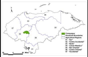
Figure 1. Study area location

3. Methodology

This research relies on two primary data sources: satellite images from 1987, 1994 and 2001, and historical recall data of farmers living in the community of Comayagua.

3.1 Land Use Change Detection

For monitoring changes in land use, Landsat digital data of August 1987 and July 1994 of Landsat 5 TM and July 2001 of Landsat 7 ETM+ has been used. The overall methodology adopted for the preparation of land use maps and change analysis is shown with the help of a flow chart in Figure 2. A modified version of the Anderson’s scheme of land use classification was adopted to make the satellite imagery interpretation and classification [1]. The categories include: 1) Urban/built-up land, 2) Cropland, 3) Pasture land, 4) Forest land (Deciduous forest, dense conifer forest, sparse conifer forest, and mixed forest), 5) Scrub land, and 6) Fallow land.

Remote sensing and GIS software was used to perform the multispectral classification, which was carried out through supervised and unsupervised classification techniques using aerial photograph and field visits as reference data. The overall accuracy of the classification was finally obtained to assess the reliability of the prepared maps.

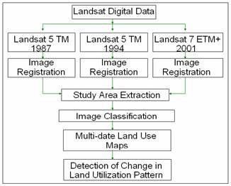
Figure 2. Methodology adopted for satellite image processing

3.2 Markov Chain Analysis of the Land Use Change Process

Imagery processing results were analyzed through the Markov chain analysis method to calculate expected transition probabilities. To apply this analysis it was assumed that the land use process constitutes a Markov process, in other words, a stochastic and random process whose different land use categories are the states of a chain [13]. The conditional probability distribution of the process at time n+1, X_n₊₁, depends only on the value of X_n, and is independent of all previous values X_n_-1, X_n_-2, . . . , X₀ that the process passes through in arriving at n. It can be expressed as:

P[X_n₊₁ = x_n₊₁ | X_n = x_n, . . . , X₀ = x₀]

= P[X_n₊₁ = x_n₊₁ | X_n = x_n] (1)

It can be also written as:

p_ij = P[X_n₊₁ = j | X_n = i] i,j = 0,1,2,… (2)

The p_ij, called the one-step transition probability, can be interpreted as the conditional probability that at time n+1 the system is in state j, given that at time n the system was in state i. When n steps are needed to implement this transition, the p_ij is then called the n-step transition probability, p_ijⁿ. This expresses the probability of transition from state i to the state j in n (>1) steps [5]. Two-steps transition probabilities can be defined and generalized to Chapman-Kolmogorov equation:

p_ij² = ∑P[X_m+n = j, X_n = k | X₀ = i]

= ∑P[X_m+n = j | X_n = k]P[X_n = k | X₀ = i] (3)

Which is equivalent to:

(P)_m+n = (P)_n ・(P)_m(4)

Applying this equation to the land use change process and with the aid of the GIS analysis functions, the expected numbers of transition probabilities were calculated using the following formula:

P_ij = (N_ik)(N_kj) (5)

Where:

N_ik represents pixels (30 m x 30m) change frequency from category i to k during the period 1987 to 1994; and

N_kj represents pixels change frequency from category k to j during the period 1994 to 2001.

3.3 Field Survey

Land use decisions are generally viewed as a function of both micro- (plot and household characteristics) and macro-level factors (community and national variables) [4]. One of the main constraints when studying these factors, particularly in developing countries, is the lack of data. Thus, in order to obtain historical recall data and study the relationship between these factors and land allocation to different uses, a land use change history survey was conducted by interviewing 30 randomly selected farmers and representatives of agriculture-related institutions in the target community.

The field survey (data of 156 plots cultivated throughout the 14-year period of study) and government publications data was used to carry out a correlation analysis to determine the direction and strength of the relationship between land use categories (land allocation) and determinant factors.

4. Results

4.1 Land Use Change

Land use maps for 1987, 1994 and 2001 were produced from Landsat 5 TM and Landsat 7 ETM+ and are depicted in Figure 3. The maps illustrate that there has been a significant reduction in forest land, which is an important concern that has continued from the past mainly as a result of traditional agriculture (slash and burn: shifting cultivation), uncontrolled urban growth, and forestry [11].

The land use change process for the target community appears in part to support the predictions of Boserup [6], who proposed that under population pressure and in absence of a frontier for expansion, people intensify agricultural production to meet subsistence needs either by expanding production at the so-called extensive margin by the creation of new fields, or by expanding production via the intensive cultivation of existing fields. This can be observed in table 1, where on the one hand, urban/built-up, cropland, scrub and fallow land have increased in area (by 159.24%, 137.88%, 72.48% and 291.08% respectively), while on the other hand, pasture and forest land have decreased in area (by 22.35% and 31.81% respectively).

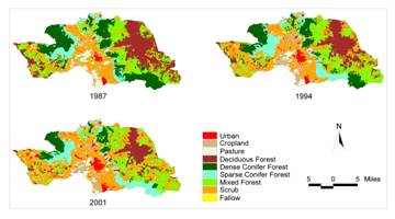
Figure 3. Land use maps, 1987 – 2001

Table 1. Land use change matrix, 1987 –2001 (ha)

1987	2001						1987 Total
1987	Urban or built-up	Cropland	Pasture	Forest	Scrub	Fallow	1987 Total
Urban or built-up	1598.67	5.13	4.68	2.43	9.27	0.00	1620.18
Cropland	193.68	1770.66	214.29	165.96	967.77	68.85	3381.21
Pasture	113.76	1277.73	1562.67	37.98	755.01	46.17	3793.32
Forest	990.63	2516.04	537.75	38589.93	15470.46	47.97	58152.78
Scrub	1300.41	2438.91	613.35	859.23	11064.51	123.84	16400.25
Fallow	2.97	34.92	12.78	1.71	20.16	1.08	73.62
2001 Total	4200.12	8043.39	2945.52	39657.24	28287.18	287.91	83421.36
Change (ha)	+2579.94	+4662.18	-847.80	-18495.54	+11886.93	+214.29	38686.68
Change (%)	+159.24	+137.88	-22.35	-31.81	+72.48	+291.08	46.37

Source: Satellite image analysis

The massive increase in urban land (159.24%) could be attributed to the rapid urban development that has taken place in the community of study during the last decade; this combined with high levels of immigration from areas less developed has caused to a certain extent an uncontrolled urban growth and reduction in forest land area. Of the 137.88 percent (4662.18 hectares) increase in cropland, 31.28% results from forest land which could indicate in part the impact of shifting cultivation practices; scrub and pasture land contribute 30.32% and 15.88% of the increase, respectively. These transitions, from scrub to cropland and pasture to cropland, could represent an indicator of land use intensification. The matrix also indicates that a great quantity of land has changed from cropland (967.77 ha) and pasture land (755.01 ha) to scrub land, which may indicate the existence of problems regarding agricultural land abandonment.

4.2 Transition Probability (TP)

In order to predict the probability that land use categories will change or remain the same in the future, expected transition probabilities between land use categories were calculated by the Markov chain analysis method and are shown in Table 2. The TPs were obtained by multiplying the transition frequency matrices of the periods 1987–1994 and 1994–2001 (see equation 5).

Table 2. Expected values of land use transitional probabilities

To From	Urban or built-up	Cropland	Pasture	Forest	Scrub	Fallow
Urban or built-up	0.96385	0.00578	0.00691	0.00719	0.01609	0.00018
Cropland	0.05153	0.38088	0.06637	0.10075	0.38223	0.01823
Pasture	0.03361	0.29526	0.36375	0.04291	0.25275	0.01174
Forest	0.01997	0.05200	0.01181	0.63957	0.27521	0.00146
Scrub	0.07136	0.15711	0.03935	0.11930	0.60706	0.00582
Fallow	0.04487	0.30373	0.09921	0.07708	0.46147	0.01365

The TPs show the probability that a land pixel will change from one land use category to another. For instance, the TP from forest land to cropland is 0.052; it means that of the total forest land pixels 5.2% may change to cropland; from cropland to scrub land 0.38223; from pasture land to scrub land 0.25275, and so forth. Hence, it can be said that important concerns such as shifting cultivation practices and land abandonment may continue, unless policies to regulate or control them are implemented.

Table 3. Correlation analysis between land use categories and determinant factors

Explanatory Variables	Irrigated Cropland	Non-irrigated Cropland	Perennial	Pasture	Forest	Fallow & Scrub
Plot level
Slope (%)	-0.058	0.115**	0.402**	-0.044	0.218**	0.009
Altitude (masl)	-0.072*	0.098**	0.247**	-0.042	0.205**	-0.034
Distance to water (km)	-0.026	0.167**	0.121**	-0.002	0.122**	-0.006
Plot area (ha)	0.494**	-0.069*	-0.042	0.746**	0.053	0.380**

Household level
Farmed area (ha)	0.653**	-0.179*	0.061	0.778**	0.133	0.477**
Farm animal (No. of animals)	0.153*	-0.169*	0.060	0.904**	0.271**	-0.034
Family labor (No. of persons)	-0.150	0.332**	-0.033	-0.184*	-0.162*	-0.002
Family size (No. of persons)	-0.010	0.154	0.031	0.218**	-0.208**	-0.185*
Education level (years of study)	0.289**	-0.295**	0.157*	0.346**	0.424**	0.432**
Migration decision (yes, no)	-0.180*	0.156*	-0.169*	-0.311**	-0.309**	-0.078

Community level
Rain fall (mm/year)	0.018	0.068	-0.028	-0.051	-0.038	0.056
Temperature (º C)	0.032	0.141	0.051	-0.051	-0.122	0.035

National level
Producer nominal price index	0.026	0.072*	0.048	-0.049	-0.066	0.040
Producer real price index	0.008	0.083*	0.017	-0.026	-0.065	0.040

* and ** indicate statistical significance at the 5% and 1% level, respectively Source: Field survey and Government publications

N = 30 farmers (156 plots)

Natural disasters and policy changes during the period concerned could have had a significant impact on the land use change of the study area. These events in addition to the community and national level variables are considered as exogenous factors, and can be summarized as follows:

1) Late 80’s – 1992. High plague incidence owing to overproduction of tomato

2) 1993. Incentives to produce Asian vegetables for export

3) 1998. Damage caused by hurricane Mitch

4) 2000 – 2001. Development of Mango processing and exporting industry

The influence of these factors on land use pattern can be seen in table 4. The relative distribution among the various land use categories at the beginning of the study period reveals that pasture land occupies approximately similar area (4.55%) compared to cropland (4.05%). However, at the end of the study period cropland increases (9.64%) and pasture land decreases (3.53%).

The decline in pasture land may be due to transitions into irrigated cropland, hurricane Mitch damages, and finally, a reduction in livestock population.

Table 4. Land use distribution during the period of study (ha)

Year	Urban or built-up	Cropland	Pasture	Forest	Scrub	Fallow
1987	1620.18 (1.94%)	3381.21 (4.05%)	3793.32 (4.55%)	58152.78 (69.71%)	16400.25 (19.70%)	73.62 (0.09%)
1994	2694.15 (3.23%)	7001.82 (8.39%)	3097.26 (3.71%)	47874.69 (57.39%)	22549.23 (27.03%)	204.21 (0.24%)
2001	4200.12 (5.03%)	8043.39 (9.64%)	2945.52 (3.53%)	39657.24 (47.54%)	28287.18 (33.91%)	287.91 (0.34%)

Source: Satellite image analysis

Although hurricane Mitch did exert a considerable impact on cropland area, it is more likely that cropland increased as a result of incentives provided to produce Asian vegetables under contract farming, immigration and creation of new traditional agriculture plots, and mango processing and exporting industry development [9].

5. Conclusion

The integration of satellite remote sensing, GIS and historical recall data provides comprehensive information to study agricultural economics related topics such as land use, allows for a better understanding of the direction, nature and rate of land use changes, and represents an alternative method to perform land use studies, especially for those areas or countries where there has been little or no long-term monitoring of agricultural management.

The land use change patterns of the study area indicate on the one hand that a positive process of land use intensification has occurred, while on the other hand, concerns such as shifting cultivation and land abandonment have increased. The Markov chain analysis confirms that these problems will continue. Farmers’ land use decisions were mainly influenced by endogenous (plot and household level) factors and policy changes.

Taking into consideration the results of the correlation analysis between determinant factors and land allocation to different uses, and the importance of education level in favoring irrigated crop development along with a reduction of shifting cultivation practices, investments in education and technical assistance programs could be of great importance for the agricultural development of the target community. On the other hand, application or reinforcing of policies such as land titling could have a positive impact on the reduction of migration levels by encouraging farmers to produce either in their area of origin or in the area where they have migrated to.

References

[1] Anderson, J. R., Hardy, E. E., Roach, J. T. and Witmer, R.E. A Land Use and Land Cover Classification System for Use with Remote Sensor Data. Geological Survey Professional Paper 964, 1976.

[2] Barbier, B., and Bergeron, G. Natural Resource Management in the hillsides of Honduras: Bio-economic Modeling at the Microwatershed Level. EPTD Discussion Paper No. 32. International Food Policy Research Institute, Washington, D.C., 1998.

[3] Bergeron, G., and Pender J. Determinants of Land Use Change: Evidence from a community study in Honduras. Environmental and Production Technology Division, International Food Policy Research Institute, Washington, D.C., 1999.

[4] Bergeron, G., and Pender J. Policy Research in Natural Resource Management Using Plot, Household, and Community Histories. Fragile Lands Program, Environmental and Production Technology Division, International Food Policy Research Institute, Washington, D.C., 1996.

[5] Bharucha-Reid, A.T. Elements of the Theory of Markov Processes and Their Applications. Dover Publications, New York, 1997.

[6] Boserup, Ester. The Conditions of Agricultural Growth: The Economics of Agrarian Change under Population Pressure. George Allen & Unwin LTD, London, 1967.

[7] Cotty, D., Estrada, I. and García, M. Indicadores Básicos sobre el Desempeño agropecuario 1971–2001. Zamorano and Instituto Nacional de Estadística, Honduras. Proyecto de Investigación en Políticas Agrícolas y Banco de Datos (AID PL - 480), 2002.

[8] Cropper, M. Regional Land Use Modeling: Past Experience and Future Directions. The World Bank, Washington D.C., 1998.

[9] Dominguez, E., and Dubon, M. R. Personal interview. 22 May 2003.

[10] International Development Research Center (IDRC). Assessment of the Political, Economic, and Institutional Contexts for Participatory Rural Development in Post-Mitch Honduras. Working Paper Series of the IDRC Program Initiative, Minga - Managing Natural Resources in Latin America and the Caribbean, 2001.

[11] Pfeffer, M. J., Schelhas, J. W., DeGloria, S. D., and Gomez J. Population, Conservation, and Land Use Change in Honduras, 2001.

[12] Ruben, R. Making Cooperatives Work, Contract Choice and Resource Management within Land Reform Cooperatives in Honduras. Centre for Latin American Research and Documentation (CEDLA), Netherlands, 1999.

[13] Weng, Q. Land use change analysis in the Zhujiang Delta of China using satellite remote sensing, GIS and stochastic modeling. Journal of environmental Management 64, 2002.