Jeffrey Jabson

FILEPR ( TH, 11-12 pm )

1.) Data Definition Language (DDL)

The schema data definition language (DDL) is used for describing a database, which maybe shared by many programs written in many languages. This description is in terms of the names and characteristics of the data items, data aggregates, records, areas, and sets included in the database, and the relationships that exist and must be maintained between occurrences of those elements in the database. l Data item. A data item is an occurrence of the smallest unit of named data. It is represented in a database by a value.

2.) Data Manipulation Language (DML)

A data manipulation language (DML) is a language used to cause data to be transferred between a run unit and the database. A DML is not a complete language by itself. It is called a query language by some manufacturers. It relies on a host language to provide a framework for it and to provide the procedural capabilities required to manipulate data.

EXAMPLES OF BOTH:

Data aggregate. A data aggregate is an occurrence of a named collection of data items within a record. There are two kinds-vectors and repeating groups. A vector is a one-dimensional sequence of data items, all of which have identical characteristics. A repeating group is a collection of data that occurs a number of times within a record occurrence. The collection may consist of data items, vectors, and repeating groups. l Record. A record is an occurrence of a named collection of zero, one, or more data items or data aggregates. This collection is specified in the schema DDL by means of a record entry. Each record entry

in the schema for a database determines a type of record, of which there may be an arbitrary number of record occurrences (records) in the database. For example, there would be one occurrence of a PAYROLL-RECORD type of record for each employee. A database key is a unique value that identifies a record in the database to a run unit (program(s)). The value is made available to the run unit when a record is selected or stored and maybe used by the run unit to reselect the same record.

Set. A set is an occurrence of a named collection of records. The collection is specified in the schema DDL by means of a set entry. Each set entry in the schema for a database determines a type of set, of which there may be an arbitrary number of set occurrences (sets) in the database. Each type of set specified in the schema may have one type of record declared as its owner type of record, and one or more types of records declared as its member type of record. Each set occurrence (set) must contain one occurrence of its defined owner type of record and may contain an arbitrary number of occurrences of each of its defined member type of record types. For example, if a set type QUALIFICATIONS was defined as having owner record type EMPLOYEE and member record types JOB and SKILL, each occurrence of set type QUALIFICATIONS must

contain one occurrence of record type EMPLOYEE, and may contain an arbitrary number of occurrences of record types JOB and SKILL. l Area. An area is a named collection of records that need not preserve owner/member relationships. An area may contain occurrences of one or more record types, and a record type may have occurrences in more than one area. A particular record is assigned to a single area and may not migrate between areas.

Database. A database consists of all the records, sets, and areas that are controlled by a specific schema. If a facility

has multiple databases, there must be a separate schema for each database. Furthermore, the content of each database is assumed to be independent. l Program. A program is a set or group of instructions in a host language such as COBOL or FORTRAN. For the purpose of this chapter, a run unit is an execution of one or more programs.

3.) System Catalog ( SYSCTLG )

In some systems, a computer file that serves as an index to all other files that the system has used or will use. The SYSCTLG shows the names, sizes, locations, and usually any other pertinent information about the files.

4.) Relational Model

The relational model was formally introduced by Dr. E. F. Codd in 1970 and has evolved since then, through a series of writings. The model provides a simple, yet rigorously defined, concept of how users perceive data. The relational model represents data in the form of two-dimension tables. Each table represents some real-world person, place, thing, or event about which information is collected. A relational database is a collection of two-dimensional tables. The organization of data into relational tables is known as the logical view of the database. That is, the form in which a relational database presents data to the user and the programmer. The way the database software physically stores the data on a computer disk system is called the internal view. The internal view differs from product to product and does not concern us here. A basic understanding of the relational model is necessary to effectively use relational database software such as Oracle, Microsoft SQL Server, or even personal database systems such as Access or Fox, which are based on the relational model.

• Normalization – definition and purpose

Normalization

Normalization is a design technique that is widely used as a guide in designing relational databases. Normalization is essentially a two step process that puts data into tabular form by removing repeating groups and then removes duplicated from the relational tables.

Normalization theory is based on the concepts of normal forms. A relational table is said to be a particular normal form if it satisfied a certain set of constraints. There are currently five normal forms that have been defined. In this section, we will cover the first three normal forms that were defined by E. F. Codd.

Basic Concepts

The goal of normalization is to create a set of relational tables that are free of redundant data and that can be consistently and correctly modified. This means that all tables in a relational database should be in the third normal form (3NF). A relational table is in 3NF if and only if all non-key columns are (a) mutually independent and (b) fully dependent upon the primary key. Mutual independence means that no non-key column is dependent upon any combination of the other columns. The first two normal forms are intermediate steps to achieve the goal of having all tables in 3NF. In order to better understand the 2NF and higher forms, it is necessary to understand the concepts of functional dependencies and loss less decomposition.

Functional Dependencies

The concept of functional dependencies is the basis for the first three normal forms. A column, Y, of the relational table R is said to be functionally dependent upon column X of R if and only if each value of X in R is associated with precisely one value of Y at any given time. X and Y may be composite. Saying that column Y is functionally dependent upon X is the same as saying the values of column X identify the values of column Y. If column X is a primary key, then all columns in the relational table R must be functionally dependent upon X.

A short-hand notation for describing a functional dependency is:

R.x —>; R.y

which can be read as in the relational table named R, column x functionally determines (identifies) column y.

Full functional dependence applies to tables with composite keys. Column Y in relational table R is fully functional on X of R if it is functionally dependent on X and not functionally dependent upon any subset of X. Full functional dependence means that when a primary key is composite, made of two or more columns, then the other columns must be identified by the entire key and not just some of the columns that make up the key.

Overview

Simply stated, normalization is the process of removing redundant data from relational tables by decomposing (splitting) a relational table into smaller tables by projection. The goal is to have only primary keys on the left hand side of a functional dependency. In order to be correct, decomposition must be lossless. That is, the new tables can be recombined by a natural join to recreate the original table without creating any spurious or redundant data.

Sample Data

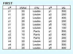
Data taken from Date [Date90] is used to illustrate the process of normalization. A company obtains parts from a number of suppliers. Each supplier is located in one city. A city can have more than one supplier located there and each city has a status code associated with it. Each supplier may provide many parts. The company creates a simple relational table to store this information that can be expressed in relational notation as:

FIRST (s#, status, city, p#, qty)

where

In order to uniquely associate quantity supplied (qty) with part (p#) and supplier (s#), a composite primary key composed of s# and p# is used.

• Anomaly – definition

Anomaly

Something contrary to the general rule as to the database, or to what is expected.

• First Normal Form – Fifth Normal Form ( 1NF, 2NF, 3NF, 4NF, 5NF )

First Normal Form

A relational table, by definition, is in first normal form. All values of the columns are atomic. That is, they contain no repeating values. Figure1 shows the table FIRST in 1NF.

Figure 1: Table in 1NF

Although the table FIRST is in 1NF it contains redundant data. For example, information about the supplier's location and the location's status have to be repeated for every part supplied. Redundancy causes what are called update anomalies. Update anomalies are problems that arise when information is inserted, deleted, or updated. For example, the following anomalies could occur in FIRST:

• INSERT. The fact that a certain supplier (s5) is located in a particular city (Athens) cannot be added until they supplied a part.
• DELETE. If a row is deleted, then not only is the information about quantity and part lost but also information about the supplier.
• UPDATE. If supplier s1 moved from London to New York, then six rows would have to be updated with this new information.

Second Normal Form

The definition of second normal form states that only tables with composite primary keys can be in 1NF but not in 2NF.

A relational table is in second normal form 2NF if it is in 1NF and every non-key column is fully dependent upon the primary key.

That is, every non-key column must be dependent upon the entire primary key. FIRST is in 1NF but not in 2NF because status and city are functionally dependent upon only on the column s# of the composite key (s#, p#). This can be illustrated by listing the functional dependencies in the table:

The process for transforming a 1NF table to 2NF is:

1. Identify any determinants other than the composite key, and the columns they determine.
2. Create and name a new table for each determinant and the unique columns it determines.
3. Move the determined columns from the original table to the new table. The determinate becomes the primary key of the new table.
4. Delete the columns you just moved from the original table except for the determinate which will serve as a foreign key.
5. The original table may be renamed to maintain semantic meaning.

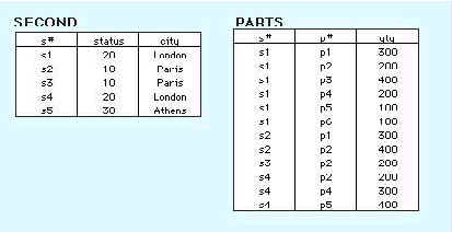
To transform FIRST into 2NF we move the columns s#, status, and city to a new table called SECOND. The column s# becomes the primary key of this new table. The results are shown below in Figure 2.

Figure 2: Tables in 2NF

Tables in 2NF but not in 3NF still contain modification anomalies. In the example of SECOND, they are:

INSERT. The fact that a particular city has a certain status (Rome has a status of 50) cannot be inserted until there is a supplier in the city.

DELETE. Deleting any row in SUPPLIER destroys the status information about the city as well as the association between supplier and city.

Third Normal Form

The third normal form requires that all columns in a relational table are dependent only upon the primary key. A more formal definition is:

A relational table is in third normal form (3NF) if it is already in 2NF and every non-key column is non transitively dependent upon its primary key. In other words, all non-key attributes are functionally dependent only upon the primary key.

Table PARTS is already in 3NF. The non-key column, qty, is fully dependent upon the primary key (s#, p#). SUPPLIER is in 2NF but not in 3NF because it contains a transitive dependency. A transitive dependency is occurs when a non-key column that is a determinant of the primary key is the determinate of other columns. The concept of a transitive dependency can be illustrated by showing the functional dependencies in SUPPLIER:

Note that SUPPLIER .status is determined both by the primary key s# and the non-key column city. The process of transforming a table into 3NF is:

1. Identify any determinants, other the primary key, and the columns they determine.
2. Create and name a new table for each determinant and the unique columns it determines.
3. Move the determined columns from the original table to the new table. The determinate becomes the primary key of the new table.
4. Delete the columns you just moved from the original table except for the determinate which will serve as a foreign key.
5. The original table may be renamed to maintain semantic meaning.

To transform SUPPLIER into 3NF, we create a new table called CITY_STATUS and move the columns city and status into it. Status is deleted from the original table, city is left behind to serve as a foreign key to CITY_STATUS, and the original table is renamed to SUPPLIER_CITY to reflect its semantic meaning. The results are shown in Figure 3 below.

Figure 3: Tables in 3NF

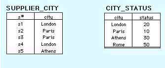
The results of putting the original table into 3NF has created three tables. These can be represented in "psuedo-SQL" as:

PARTS (#s, p#, qty)
Primary Key (s#,#p)
Foreign Key (s#) references SUPPLIER_CITY.s#

SUPPLIER_CITY(s#, city)
Primary Key (s#)
Foreign Key (city) references CITY_STATUS.city

CITY_STATUS (city, status)
Primary Key (city)

Advantages of Third Normal Form

The advantages to having relational tables in 3NF is that it eliminates redundant data which in turn saves space and reduces manipulation anomalies. For example, the improvements to our sample database are:

INSERT. Facts about the status of a city, Rome has a status of 50, can be added even though there is not supplier in that city. Likewise, facts about new suppliers can be added even though they have not yet supplied parts.

DELETE. Information about parts supplied can be deleted without destroying information about a supplier or a city. UPDATE. Changing the location of a supplier or the status of a city requires modifying only one row.

Advanced Normalization

After 3NF, all normalization problems involve only tables which have three or more columns and all the columns are keys. Many practitioners argue that placing entities in 3NF is generally sufficient because it is rare that entities that are in 3NF are not also in 4NF and 5NF. They further argue that the benefits gained from transforming entities into 4NF and 5NF are so slight that it is not worth the effort. However, advanced normal forms are presented because there are cases where they are required.

Boyce-Codd Normal Form

Boyce-Codd normal form (BCNF) is a more rigorous version of the 3NF deal with relational tables that had (a) multiple candidate keys, (b) composite candidate keys, and (c) candidate keys that overlapped .

BCNF is based on the concept of determinants. A determinant column is one on which some of the columns are fully functionally dependent.

A relational table is in BCNF if and only if every determinant is a candidate key.

Fourth Normal Form

A relational table is in the fourth normal form (4NF) if it is in BCNF and all multi-valued dependencies are also functional dependencies.

Fourth normal form (4NF) is based on the concept of multi-valued dependencies (MVD). A Multi-valued dependency occurs when in a relational table containing at least three columns, one column has multiple rows whose values match a value of a single row of one of the other columns. A more formal definition given by Date is:

given a relational table R with columns A, B, and C then

R.A —>> R.B (column A multi determines column B)

is true if and only if the set of B-values matching a given pair of A-values and C-values in R depends only on the A-value and is independent of the C-value.

MVD always occur in pairs. That is R.A —>> R.B holds if and only if R.A —>> R.C also holds.

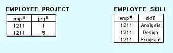
Suppose that employees can be assigned to multiple projects. Also suppose that employees can have multiple job skills. If we record this information in a single table, all three attributes must be used as the key since no single attribute can uniquely identify an instance.

The relationship between emp# and prj# is a multi-valued dependency because for each pair of emp#/skill values in the table, the associated set of prj# values is determined only by emp# and is independent of skill. The relationship between emp# and skill is also a multi-valued dependency, since the set of Skill values for an emp#/prj# pair is always dependent upon emp# only.

To transform a table with multi-valued dependencies into the 4NF move each MVD pair to a new table. The result is shown in Figure1.

Figure 1: Tables in 4NF

Fifth Normal Form

A table is in the fifth normal form (5NF) if it cannot have a lossless decomposition into any number of smaller tables.

While the first four normal forms are based on the concept of functional dependence, the fifth normal form is based on the concept of join dependence. Join dependency means that an table, after it has been decomposed into three or more smaller tables, must be capable of being joined again on common keys to form the original table. Stated another way, 5NF indicates when an entity cannot be further decomposed. 5NF is complex and not intuitive. Most experts agree that tables that are in the 4NF are also in 5NF except for "pathological" cases. Teorey suggests that true many-to-many-to-many ternary relations are one such case.

Adding an instance to an table that is not in 5NF creates spurious results when the tables are decomposed and then rejoined. For example, let's suppose that we have an employee who uses design skills on one project and programming skills on another. This information is shown below.

Next we add an employee (1544) who uses programming skills on Project 11.

Next, we project this information into three tables as we did above. However, when we rejoin the tables, the recombined table contains spurious results.

By adding one new instance to a table not in 5NF, two false assertions were stated:

Assertion 1

• Employee 1211 has been assigned to Project 11.
• Project 11 requires programming skills.
• Therefore, Employee 1211 must use programming skills while assigned to Project 11.

Assertion 2

• Employee 1544 has been assigned to project 11.
• Project 11 needs Design skills.
• Therefore, Employee 1544 must use Design skills in Project 11.

BACK