This document introduces you to the MatlabR12.x suite of applications from Mathworks, Inc. The R12.x release consists of version 6.x of the primary Matlab application along with some auxiliary modeling and simulations applications and specialized toolboxes. The suite as a whole will be surveyed but the primary application, Matlab 6.x, will be the focus of this tutorial. Instruction is aimed toward first-time users; however, those who are already familiar with previous versions of Matlab can use this document to learn about some of Matlab's new features. The document is organized into six sections. The first section provides a brief introduction to this tutorial and to Matlab. The second section gives an overview of the Matlab desktop layout and guides the reader through each of the windows and their functions. Also covered in this section is the layout for the built-in Matlab Help. The third section covers the basic methods of getting data into and exporting data from Matlab, including the import wizard, command line I/O functions, and M-books. A fourth section concerns the interactive functionality of Matlab, including elementary mathematical and matrix operations. A fifth section will introduce the Matlab programming language and the construction of M-files, which are callable scripts, macros, and functions that can be used from the Matlab command line prompt or can be nested within another such file. The sixth and final section briefly covers built in demo scripts that illustrate some of the types of problems for which Matlab is a useful application, including the use of the auxiliary Simulink utility for constructing and simulating a dynamical model. Also, this section will introduce the usage of Matlab Toolboxes, which are ensembles of related M-files developed for specific types of applications.
Introduction to Version 6.x of Matlab
In the 1960s and 1970s before the appearance of personal computers, complex and large scale calculations were done on large mainframes using code primarily developed with Fortran. As a number of related large subroutines were developed for specific computational purposes, they were organized into public domain packages and distributed for free. Matlab was originally created as a front end for one of these, the LINPACK package -- a group of routines for working with matrices and linear algebra. The primary developer, Professor Cleve Moler at the University of New Mexico, eventually founded Mathworks, Inc., to further develop and market the product in a commercial setting. From the original Matlab, a high powered suite of applications has evolved. The latest release, MatlabR12.x, features the newest kernel, Matlab 6.x. It is largely backward compatible with recent Matlab versions, but there are some slight syntax changes. The biggest changes that users of earlier versions of Matlab will notice are the implementation of a desktop layout format for interactive use and differences in the handle graphics that now accommodate several point and click features for labeling and enhancing plots and graphical output.
Section 2: An Overview of Matlab 6.x
Information Technology Services (ITS) at UT-Austin provides free Matlab 6.x access to students, faculty or via the desktop computers in the Student Microcomputer Facility (SMF) on the second floor of the Flawn Academic Center (FAC 212). Before using these machines it will be necessary to have an individually funded (IF) or departmental sponsored account issued by ITS. A basic account that can be used in the SMF has no cost, though there will be some service charges if optional validations for internet dialup service or mainframe disk storage allocation is desired. Information about getting an ITS- issued account is available at
http://www.utexas.edu/cc/account/index.html
There are also installations of Matlab 6.x on the three ITS Unix systems: ccwf.cc.utexas.edu which runs on Solaris 2.6, uts.cc.utexas.edu which runs on Digital Unix, and spice.cc.utexas.edu which runs on AIX. A Windows version of Matlab 6.x is installed on the ITS Windows NT terminal server, earthquake.cc.utexas.edu. To access these installations, an ITS-issued account must have HPW validation (ccwf), UTS validation (uts), ADS validation (spice), or WNT validation (earthquake). These mainframe validations require a minimum of 1000K disk storage costing 3 cents per day.
Some academic departments (e.g., Chemical Engineering) also have Matlab 6.x already installed on machines in their local computer labs. Also, other UT-Austin departments are eligible to purchase licenses for Matlab 6.x for use within their own labs through the Software Distribution Services unit of ITS. Details of various licensing options available for purchase by academic departments are available at
http://www.utexas.edu/cc/sds/products/matlab.html
The MatlabR12.x suite containing Matlab 6.x is also marketed directly by Mathworks, Inc., which has special academic pricing and, for individuals enrolled as students, a very inexpensive student edition with full functionality. Information and pricing is given at
http://www.mathworks.com/store/index.html
The procedure for launching Matlab 6.x is no different from that used with earlier versions. However, the launch method varies.
If the Matlab application is being run on a remote X terminal using a Unix mainframe application, then the DISPLAY variable has to be set to the local terminal and the local terminal has to grant access to the Unix mainframe. Both of these requirements can be circumvented if the mainframe connection is through a secure shell (SSH) protocol. Otherwise the commands setenv DISPLAY myhost.mydomain:0.0 and xhost +remotesystem.remotedomain will need to be executed at the shell prompt. Matlab 6.x can then be started at a shell prompt with the command matlab, or, in background with concurrent access to other processes with the command matlab &.
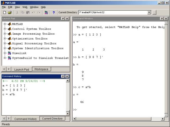
Once the path environment is set properly and the desktop appears on the monitor screen, using Matlab 6.x will be practically the same for all operating system distributions. There are several windows that can be used in arranging the desktop, but a default configuration will appear upon launching. If desired this can be modified by selecting an alternate choice from View -> Desktop Layout . The default desktop has a small Current Directory selection window near the top, with the Work folder being specified initially. If other folders have been added, then another current directory setting can be selected from among those available. The main area has the Command window on the right and an upper and lower pair of toggled windows on the left side. The upper left panel will show the Launch Pad window which can be toggled with a Workspace window. The lower left panel will show a Command History window and can be toggled with a Current Directory window. There are also remote Help and Demo windows that can be launched from the Desktop�s Help pull down menu. Also there is a remote Figure window that is launched whenever a command involving graphical display is executed.
The Launch Pad window, displayed in the upper left of the default desktop configuration, serves as a convenient assemblage of shortcuts to common operations and windows that may not currently be displayed. For example, the Help window can be launched by clicking on the icon here rather than using the navigation bar pull-down menu. A Demo window for demonstrations can be launched from here, as can auxiliary applications such as Simulink.
The Workspace window provides an inventory of all the items in the workspace that are currently defined, either by assignment or calculation in the Command window or by importation with a load command from the Matlab command line prompt.
The Command History window, at the lower left in the default desktop, contains a log of commands that have been executed within the Command window. This is a convenient feature for tracking when developing or debugging programs or to confirm that commands were executed in a particular sequence during a multistep calculation from the command line.
The Current Directory window displays a current directory with a listing of its contents. There is navigation capability for resetting the current directory to any directory among those set in the path. This window is useful for finding the location of particular files and scripts so that they can be edited, moved, renamed, deleted, etc. The default current directory is the Work subdirectory of the original Matlab installation directory.
The Command window is where the command line prompt for interactive commands is located. This is also the only window that appears if you execute the Unix version of Matlab outside of an X environment, e.g., on a vt100 screen. Commands and scripts can be executed from a vt100 window, but graphics and desktop tools will not be available. The Matlab prompt on the command window consists of two adjacent right angle brackets, i.e., >>. Results of command operations will also be displayed in this window unless the command line is terminated by a semi-colon, in which case the display of results is suppressed. If a command or script specified on the command line is questionable or cannot be executed because of invalid syntax, undefined variables, etc., a diagnostic message will be displayed in the Command window. The current value of any saved variable is also displayed in this window if its name is entered at a prompt.
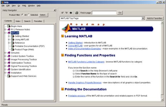
Separate from the main desktop layout is a Help desktop with its own layout. This utility can be launched by selecting Help ->MATLAB Help from the Help pull down menu. This Help desktop has a right side which displays the text for help topics, organized as tutorial of sorts. The left side has various tabs that can be brought to the foreground for navigating by table of contents, by indexed keywords, or by a search on a particular string.
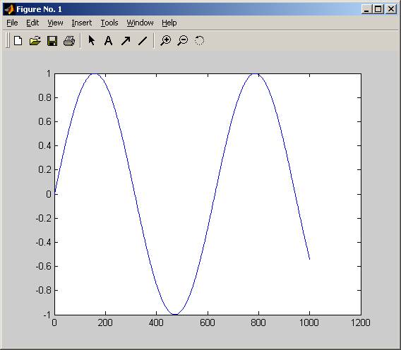
There is a Figure window that floats independently from the main desktop. If not already present, it is launched when command execution results in graphical output. From the Edit menu on the main toolbar, there are selections for editing figure properties, axis properties, and properties of objects within figures. On the Tools menu of the main toolbar there are selections for further manipulation such as zooming and perspective rotation. There is also a main toolbar menu for Help, which includes specific graphics help and demos.
 +
+
Section 3: Importing and Exporting Information
Information can be imported into and exported from the Matlab application by several different methods. Some of the more common procedures are discussed below. Command Line Import
The most
elementary method for importing external information is piece by piece directly
from the command line by typing at the keyboard. For example:
>>
earthradius = 6371
will assign
the numerical value 6371 to a variable earthradius. For
extensive amounts of information there are more efficient methods.
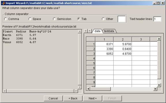
Matlab-6.x provides an Import Wizard for convenient importation of data from external files. This tool can be activated by selecting File -> Import Data, or by executing the command
>>
uiimport
at a Matlab command line prompt. This utility can be used for importing both text and numerical data contained within the same data file, but entries have to be in a matrix format with specified column separators. As an example, consider a small file, planetsize.txt, containing a few planets� names, radii, and masses with columns separated by tabs:
Planet Radius Mass-kg*10^24
Earth
6371
5.97
Mars 3390 0.64
Venus 6052 4.87
This file can be selected from the import wizard window as shown below
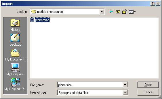
Clicking Open will import the file into Matlab. A preview screen appears which lets you confirm the data importation, with separate tabs to examine the numerical data and the text fields:
To continue, click on Next> and a new screen will provide the opportunity to selectively choose which information from the file to import into the Matlab workspace. The process is completed by clicking Finish .
There are a
variety of other ways to import complex data using the Command Window. Below several of these functions are
described in detail. csvread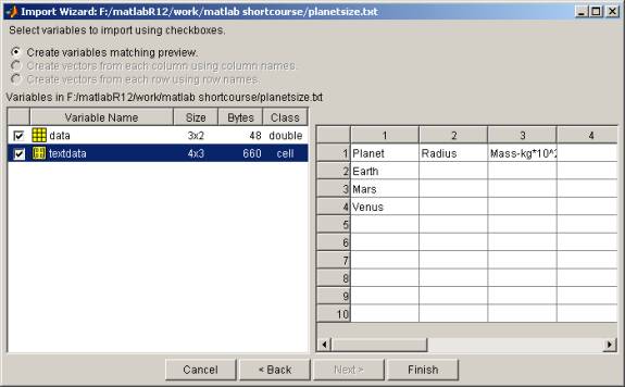
This
function imports numeric data with comma-separated values (csv). For example, in the planetary data
above, suppose that we have an external file planets1.txt ,
containing the kilometer radial distances and 10^24 kg mass values for Earth,
Mars and Venus:
6371,5.97
3390,0.64
6052,4.87
The
command
>>
planets1 = csvread('planets1.txt')
would
create a 3x2 matrix with the name planets1 whose
content is the same as that shown on the data tab generated previously (see page
11) by using the import wizard for
dlmread
This
function is similar to csvread but more
flexible, allowing the delimiter to be specified by any character rather than
restricting it to be a comma. For
example, suppose that the file planets2.txt
had the
format
6371;5.97
3390;0.64
6052;4.87
where values
are separated by semi-colons. The
command
>>
planets = dlmread('planets2.txt', ';')
would
create that same 3x2 matrix with the name
planets2.
load
This is
similar to csvread and
dlmread but the
separators have to be blank spaces.
For example, if the file planets3.txt has the
structure
6371
5.97
3390
0.64
6052 4.87
then the
command
>>
load planets3.txt
would create
the same 3x2 matrix with the name planets3.
fscanf
This is a
lower level import function, equivalent to the C language function of the same name but
with the important difference that the result is vectorized. It requires extra manipulations of
opening and closing the file, but is more versatile in allowing text and numbers
to be read in together. For
example, if we want to import the data from our file planetsize.txt we could
use the following sequence of commands to import the contents of the file in
vectorized form
fid
=fopen('planetsize.txt');
planetsize
= fscanf(fid,'%c')
fclose(fid);
where the
'%c' argument for fscanf is identical to the C language, i.e.,
parsing as character strings. The
variable planetsize is then
actually an 80 element row vector of characters (including blank spaces, tabs,
and linefeeds) which have numerical ascii character code values. Characterized data values need to be
converted to numbers before mathematical manipulations will make sense. For example, we could convert the
characters in the string representing the earth radius, i.e., elements 39 � 42,
to numerical form using the str2num Matlab function:
>>
earthradius =
str2num(planetsize(39:42))
The variable
earthradius will be in
numerical form, ready for performing mathematical operations, e.g.,
>>
earthvolume = (4/3)*pi*((earthradius)^3)
textread
The
textread function is
similar to the primitive fscanf
but will
allow data variables to be defined as part of the import process. As an example, again suppose that
the file planetsize.txt contains
the information that we want to import into Matlab. We can specify the number of
header lines to skip before reaching the actual data (one such line in this
example), and the individual data formats for each column of data. The file contains the character string
planet names in the first column, the decimal integer planet radii in the second
column and the floating point planet masses in the third column. Thus, the command
>>
[planets, radii, masses] = textread('planetsize.txt', ...
'%s %d
%f','headerlines',1)
where "%s"
signifies string, "%d" signifies decimal, and "%f" signifies floating point in
the format argument, will give the display
planets =
'Earth'
'Mars'
'Venus'
radii
=
6371
3390
6052
masses
=
5.9700
0.6400
4.8700
and add the
vector variables planets,
radii, and masses to the
workspace.
diary
The simplest
way to export data to an external file is make use of the diary function. This is a utility for logging a
transcript of the Matlab command line input and screen output. The logging process starts subsequent to
the command
>>
diary
filename
where
"filename" is chosen, and terminates with the command
>>
diary off
thus
creating an external file that can be edited with a text editor to remove
extraneous material. For an
example, let us create new variables using the data imported from the
planetsize.txt file:
>>
volumes = (4/3).*pi.*((radii).^3);
>> densities =
(10^27).*masses./((10^15).*volumes);
>> planetinfo(:,1) =
volumes;
>> planetinfo(:,2) = densities;
The
variable
planetinfo
will then be
a 3 x 2 matrix with column 1 containing planet volumes in cubic kilometers and
column 2 containing planet densities in grams per cubic centimeter. To export this information to an
external file planets4.txt
we first
activate the diary, set the display format to exponential form, type in the name
of the variable planetinfo, and turn
off the diary:
>>
diary planets4.txt
>> format short e
>> planetinfo
>> diary off
The
external file planets4.txt then contains
format
short e
planetinfo
planetinfo
=
1.0832e+012 5.5114e+000
1.6319e+011 3.9219e+000
9.2851e+011 5.2450e+000
diary
off
The planets4.txt
file can then be put into a text editor
for deleting unwanted lines, adding column headers, etc.
dlmwrite
The
dlmwrite
function allows you to write external data files in which the delimiter
can be specified. Let us assume
that we have the variables from the textread example
above on page 14 loaded into the workspace; that we have defined the vector
variables volumes and
densities
as shown on
that same page ; and that we want to write out a new file planets5.txt with the new volume and density
data. We create a local
array planets5 in the
Command Window by typing in the
desired data, a column for each of the two vector variables
>>
planets5(:,1) = volumes;
>> planets5(:,2) = densities;
The command
dlmwrite('planets5.txt',planets5,
'; ')
requests
that the contents of the array planets5
be written
to an external file planets5.txt using a
semicolon delimiter. Thus the new
external file planets5.txt will
contain
1083206916845.75;5.5114
163187806143.123;3.9219
928507395798.201;5.245
save
This utility
is a primitive function that will save an array in an external file with columns
separated by blank space.
With no arguments at all, the
save
command will
store the current values of all variables in a binary file matlab.mat
from which they can be retrieved in a subsequent Matlab
session. Using the same array
planets5 created
above, the command
>>
save planets5.txt planets5 -ascii
will produce
an external file
planets5.txt whose
content is
1.0832069e+012 5.5114124e+000
1.6318781e+011 3.9218617e+000
9.2850740e+011 5.2449771e+000
Without an
extension such as ".txt" and the flag "-ascii", the default external file will
be given a default extension ".mat" and will be in binary format.
fprintf
This is
another low level function that is equivalent to the C language function of the
same name. It is useful for
exporting information that contains both text and data in a specified format,
using syntax similar to that of the C programming language. As an example, suppose we want to export
the newly computed planet volume and density values
shown on page 15 into a file
planetinfo.txt
that has the same layout as the imported
file planetsize.txt. For this purpose we need to
create strings of 49 characters for each line in a new array, both the header
line which identifies the data in each column and the three subsequent data
lines themselves. We will give the
new 4x49 array the arbitrary name outdata. The header for the column of planet names,
consisting of the first ten characters of each line, can be created by
assignment
>>
outdata(1,1:10) = 'Planet
'
and
the headers for the the variable
columns, spanning 38 subsequent
characters, can be generated
by
>>
outdata(1,11:48) = 'Volume (km^3)
Density(g/cc) '
The
subsequent data lines will have the planet names and variable values. For these, the numeric values in the
planetinfo
variable need to be
converted to text using the Matlab num2str
utility. For example
>>
outdata(2,1:10) = 'Earth
'
>> outdata(3,1:10) = 'Mars '
>> outdata(3,11:48) = num2str(planetinfo(2,:))
>> outdata(4,1:10) = 'Venus '
>> outdata(4,11:48) = num2str(planetinfo(3,:))
We also need
to create an end of line character for each line in the 49th
position. This is done using the
Matlab sprintf
command,
which functions as a printing command in the same way as its namesake does in
the C programming language
>>
outdata(1:4,49) = sprintf('\n')
where "\n"
is the notation for the end-of-line character. As an output format we want the
text strings with a line feed in the display wherever there is an end-of-line
character in the array. We can
create a format variable, for example outformat, which
specifies the display characteristics by assigning it a string value with parsing
instructions
>>
outformat = '%s \n'
where "%s"
indicates a string and "\n" indicates a linefeed at the end-of-line
character. The new file with the
derived variable data can then be created with a sequence of two commands, the
first opening a new file with fopen and
assigning it a numerical file ID and the second printing the contents in the
desired format with fprintf, both of
which are analogous to their namesake commands in the C programming language.
In our
example we created the output array by row whereas fprintf assembles
by column. Thus the array that we
want exported is actually the transpose of that which we created, i.e.,
outdata' (with the trailing single quote mark)
rather than outdata
itself. In the Command Window we
therefore execute the commands
>>
fid = fopen('planetinfo.txt', 'w')
>>
fprintf(fid,outformat,outdata')
where the
"w" is the permission argument of fopen signifying
permission to create and write to the file.
A sequence
of command line instructions can be assembled as a macro for use in importing
information. These are called "m
files" and have file names with the extension ".m". For example, an external M-file planetradii.m containing
earthradius
= 6371
marsradius = 3390
venusradius = 6052
can be used
as a source to import these variables with these values using the command
>> planetradii
The
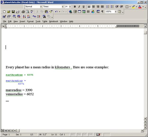
M-Book feature is
new to Matlab version 6.x. It is
used to transfer data between Matlab and Microsoft Word, a commonly used word
processing utility. As an example,
suppose that we have a small Microsoft Word document with the name planetdata.doc containing the following text
Every planet has a
mean radius in kilometers. Here are some examples: earthradius = 6371 This file can be
imported into Matlab as an M-book, but if the notebook utility has not been used
before, the setting first needs to be configured. With the command >> notebook
-setup Matlab will prompt for a
version of Microsoft Word, its file location and the location of a template to
be used for the M-book file. If this configuration is already in place, the
command >> notebook
planetdata.doc is used to access
the external file. If no Microsoft
Word file exists yet, one can be created using the generic command >> notebook which opens up a
blank Microsoft Word document; followed by Insert -> File and navigating to the
location of planetdata.doc. This procedure also adds a Notebook pull down menu to the Word toolbar. Once imported, cells can be defined and
evaluated within the document by making the appropriate selections from the Notebook pull down menu on the toolbar. In addition
to the basic methods presented in this tutorial, there are several utilities
available in Matlab for importing specialized types of binary files. Examples are aviread for
audio-video interleaved (AVI) files,
imread
for image files in common formats such as
.jpg or .gif, and xlsread for Excel spreadsheets. Section 4: Numerical and
Data Manipulation
The basic element that MATLAB
(MATrix LABoratory) uses is the matrix of numbers (real or complex). Loosely
speaking, a matrix is any orthogonal arrangement of objects (in our case
numbers), for example: A
matrix in Matlab is represented by its elements ordered in rows and columns and
included in brackets [ ]. Note also, that Matlab views any number as a matrix
with exactly one element; that is, 3 in Matlab is the same as [3]. To define a
matrix from the command window, list the matrix rows, each separated by a
semicolon. For example to define the matrix A
above: >> A=[1 -2 3.4; 7 8.3 -9]
ans = >> A(1,2) ans =
-2 In the following section the
basic matrix operations are described. Matrix Transpose The most elementary operation we
examine is the transposition of a matrix. Essentially, by interchanging the
roles of rows In Matlab the quotation mark
' is used to denote the transpose. For example:
>> A=[1 2 3; >> A' ans = that
is, elements belonging to the same rows and columns are added (or subtracted),
to produce the elements of the matrix A+B (or A-B ) . For example: >> A=[1 -2 3.4;7 8.3 -9] A = >> B=[1 3 5;2 4 6] B = >> A+B ans = >> A-B ans = Multiplying
Matrices In other words, we just need to
multiply each element of A by the constant c
to obtain the matrix cA. In
Matlab the notation c* A
is used. For instance:
>> A=[ 9 2 1.1 ; 4 6.7 0] A = ans =
Defining the product AB
of two matrices is more complicated and not intuitively obvious (the
reasoning of why we define multiplication of matrices as follows is outside of
the scope of this introductory course). One important condition must be met
before we can multiply matrix
A by B. The number of columns in A
must be the same as the number of rows in B, in other words A
has the size n by
m and B
has the size m by
k. Then the matrix product is defined by: and it is an n
by k matrix. Matlab uses the asterisk symbol
for Matrix multiplication ( A*B ). >> A=[1 2; 3 4] A = >> B=[1 3 4 5; 6 0 1 2] B = >> A*B ans =
>> A=[0 0; 1 2] A = >> B=[-1 -1;3 4] B = >> A*B ans = >> B*A ans =
>> A=[1 2; 3 4] A = >> A^3 ans =
where A
and B must have exactly the same size.
It is a generalization of the inner (or dot) product of two vectors which is
frequently used in Analytical Geometry. The symbol .* is used in Matlab for this operation.
For example: >> A=[1 5;2 6;3 7;4 8] >> B=[0 -1;1 3;0 2;2 0] B = >> A.*B ans =
In a similar fashion we use
element-wise multiplication in order to raise matrix A
to the power of B. If A
and B possess the same dimensions, the
operation is defined as follows: >> A=[1 2;5 6] A = >> B=[3 4;0 -1] >> A.^B ans =
Dividing Matrices In order to divide matrices , we
must first define the identity matrix I and the inverse
matrix. The identity matrix plays the same role as does the unity among real or
complex numbers, that is if you multiply
A by I
the product is still A. In
an n by
n identity matrix , all
non-diagonal elements are equal to zero, and all diagonal elements are equal to
one. Formally it is defined by: where It
is easy to verify that AI=IA=A for any square matrix A. The Matlab command eye is used
to construct identity matrices. The number in parentheses specifies the size of
the desired identity matrix. For example: >> eye(3) ans =
Next
suppose that A and B
are n by
n matrices such that AB=BA=I. In this case B
is called the inverse of
A and we use the
symbol A-1 to denote it. The corresponding
Matlab command is inv. In the following example we compute the inverse of
a matrix and verify that it indeed
satisfies the identity AA-1=A-1A=I .
>> A=[-1 2 4; 6 4 0;1 3 7] >> inv(A) >> A*ans ans = >> inv(A)*A ans = (Note in the last example the use
of the variable ans. By default, ans contains the last value
computed by Matlab). Next we examine the two kinds of matrix division that
Matlab handles. Suppose that B is a square matrix such that its inverse
exists. Then the quotients of
A divided by B, from the right and left, are defined
respectively by: where of
course the size of A must be such that the
expressions AB-1 or B-1A make
sense. For these operations we use the commands A/B and
B\A respectively. For
example: >> A=[0 1;1 2] A = >> B=[5 6;0 3] B = >> A/B ans = >> B\A ans =
Using
matrices we are able to rewrite the system in the more compact form where To solve
for x, we can multiply from the left both sides of the equation
by A-1 then using the
properties A-1A=I and IA=A , we
infer x=A-1b . Hence, in order to compute the
solution using Matlab, we just need
to exploit the command A/b.
For example, suppose we want to solve the system: Here, Then, we
use the following steps in the Command Window to evaluate the
solution: >> A=[2 3 4;5 -7 6;10 5 3] A = >> b=[1
marsradius = 3390
venusradius = 6052
Basic
Operations
![]()
A
line break may also be used as a row delimiter:
>>A=[1 -2 3.4 ; 7
8.3 -9]
1.0000 -2.0000 3.4000
The size of a matrix is defined by a pair of numbers; the first is
the number of its rows and the second the number of its columns. We say
that A is an n
by m matrix to indicate that A
has n rows and m
columns. The command size returns the
size of a matrix. For this example:
>> size(A)
2 3
Knowing the size of a matrix
permits us to locate any of its elements precisely by just identifying the row
and column in which it belongs. For example, the element -2
of A lies on its first row and second column
and hence can be identified by the pair of indices (1,2). Symbolically, we write
A12=-2 .
Similarly A23=-9 ,and so forth. In Matlab, any
element of a matrix is declared by typing
A(i,j), where i and j are the row and column in which the element
lies. For example:
and columns of an
n by m
matrix A we obtain a new m
by n matrix, denoted
by AT . More precisely, the
transpose AT
is defined as follows: ![]()
4 5 6
2
5
3 6
1.0000 -2.0000 3.4000
7.0000 8.3000 -9.0000
1 3 5
2 4 6
2.0000 1.0000 8.4000
9.0000 12.3000 -3.0000
0 -5.0000 -1.6000
5.0000 4.0000
-15.0000
![]()
9.0000 2.0000 1.1000
4.0000 6.7000
0
>> 2*A
18.0000 4.0000 2.2000
8.0000
13.4000
0
![]()
As an example:
1 2
3 4
1 3 4 5
6 0 1 2
13 3 6 9
27 9 16 23
Interestingly, matrix
multiplication is not commutative; that is, in general AB
is not equal to BA. For
example:
0 0
1 2
-1 -1
3 4
0 0
5 7
-1 -2
4
8
In a more general setting,
multiplying a square matrix A, by
itself n times results in a power
matrix An . In Matlab the convention A^n is used to denote this operation. For
instance:
1 2
3 4
37 54
81 11
![]()
1 5
2 6
3 7
4 8
0 -1
1 3
0 2
2 0
0 -5
2 18
0 14
8 0
![]()
1 2
5 6
3 4
0 -1
1.0000 16.0000
1.0000
0.1667
![]()
![]()
1 0 0
0 1 0
0
0 1
6 4 0
1 3 7
0.7500 0.1964 -0.4286
-0.2500
-0.0893
0.2857
0
1.0000
0
0
0
1.0000
1.0000
0
0
0 1.0000
0
0
0
1.0000
0 1
1 2
5 6
0 3
0 0.3333
0.2000 0.2667
-0.4000 -0.6000
0.3333 0.6667
![]()


![]()
![]() .
.


5 -7 6
10 5 3
0
-1
>> x=A\b
x =
-0.2349
0.0896
0.3002
As in the multiplication case, it is straightforward to define element-wise division of matrices, in the following manner:
![]()
where
matrices A and B
have the same size. In Matlab we use the notation A./B for this operation. For
example:
>> A=[1 3
4 5
>> B=[-1 -2
-5 8
>> A./B
ans =
-0.8000 0.6250
These are the very basic matrix operations that Matlab can handle. Further information about the sophisticated tools that Matlab offers can be found in the elmat.m, matfun.m and sparfun.m files accompanying Matlab (type help elmat, help matfun or help sparfun in the command line) or online at the URLs :
http://www.mathworks.com/products/matlab/functions/specialized_matrices.shtml
http://www.mathworks.com/products/matlab/functions/matrix_functions_nla.shtml
http://www.mathworks.com/products/matlab/functions/sparse_matrix.shtml
Matlab provides a rich variety of built-in functions frequently encountered in engineering and mathematical applications. In this section we describe the most elementary ones, which are taught in introductory Calculus courses. We also show how to plot the graphs of them by making use of the command plot.
For a power function we use the
hat symbol ^ (recall the
powers of matrices in the previous section). For example to evaluate the
function 1.3x at x=1, 4, 5, 6, we use the
following command:
>> 1.3.^[1 4 5 6]
ans =
1.3000
2.8561
3.7129
4.8268
Note that using a matrix as an input to 1.3x prevents sequential evaluation of the function for each value of x, on the part of the user.
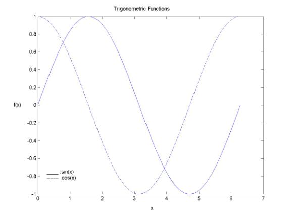
The commands for sine, cosine and
tangent functions are sin, cos, tan respectively. Also Matlab has
a built-in constant pi for the value of
pi=3.14159� . As an example:
>> sin([0 pi/4 pi/2 3*pi/4 pi])
ans =
0 0.7071 1.0000 0.7071 0.0000
>> cos([0 pi/4 pi/2 3*pi/4 pi])
ans =
1.0000 0.7071 0.0000 -0.7071 -1.0000
>> tan([0 pi/3 2*pi/3 pi])
ans =
0 1.7321 -1.7321 -0.0000
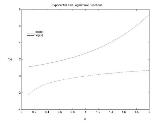
The commands for the
exponential and logarithmic (with respect to the basis e=2.71828�) functions are
exp and log respectively. As an example:
>> exp([0 1 2 3 4])
ans =
1.0000 2.7183 7.3891 20.0855 54.5982
>> log([1 2.7183 7.3891 20.0855
54.5982])
ans =
0 1.0000 2.0000 3.0000 4.0000
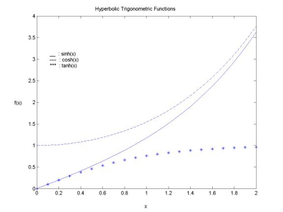
The
last set of functions we examine are the hyperbolic trigonometric functions. The
commands for the hyperbolic sine, cosine and tangent are sinh, cosh and
tanh respectively. For example:
>> sinh([0 1 2 3])
ans =
0 1.1752 3.6269 10.0179
>> cosh([0 1 2 3])
ans =
1.0000 1.5431 3.7622 10.0677
>> tanh([0 1 2 3])
ans =
0 0.7616 0.9640 0.9951
Our next task is to plot the graphs of these functions. This can be accomplished by utilizing the command plot, which is used for two dimensional graphs. The syntax of the command is
plot( x,y,'-')
where x and y are vectors containing the x and f(x) values respectively (the '-' string is used to define the plotting format). For example, the command
plot( [0:0.1:7] , sin( [0:0.1:7] ) , '-' )
plots the graph of sin(x) defined on the closed interval [0,7]. Here, [0:0.1:7] is a compact way to write the vector containing all values from 0 to 7 with an increment of 0.1 . Should a more accurate graph be needed, the increment has to be smaller. In the sequel we present the graphs of the example functions of this section.
Further information on advanced topics about Matlab built-in functions can be found in the elfun.m, specfun.m, polyfun.m help files (type elfun, specfun, or polyfun in the command line) or on the Mathworks web-page:
http://www.mathworks.com/products/matlab/functions/elem_math.shtml
http://www.mathworks.com/products/matlab/functions/spec_math.shtml
http://www.mathworks.com/products/matlab/functions/polynomial.shtml
Basic Language
Structure
Interactive Input/ Output
algorithms before implementing them using a higher-level programming language. Another obvious advantage for using Matlab is that a separate graphics package is not required for visualization of program results. Running and debugging Matlab scripts is easily done through the Matlab editor (Type edit in the command line or click the New M-File button on the Matlab-Desktop to open it- See next figure).
Let's begin with the basic interactive Input/ Output commands. To assign a value to a variable interactively we use the command input, which has the structure var=input('string'). Here, var is the variable to be assigned a value and string is an auxiliary message for the user. When the command is executed, the program waits for a value from the user (type a value for var and press return) and then proceeds to the next command. For example:
>> v=input('Input vector v \n')
Input vector v
[1 2 3 4]
v =
1 2 3 4
To
print a string on the screen we use the command fprintf, which has the
simple structure fprintf( 'string' ). For example:
>> fprintf('Matlab Short Course')
Matlab Short Course
As we have already seen, to print
matrix A on the screen we just have to type A. This results in the appearance of
the name of the matrix along with its elements. To print only the matrix
elements we use the command disp. For example:
>> A=[1 2 3; 4 5 6]
A =
1 2 3
4 5 6
>> disp(A)
1 2 3
4
5 6
Special Symbols / Logical
Operators
|
; Suppresses command output |
|
% Add comment |
|
= Value assignment |
|
< , > Order symbols |
|
= = Logical equality |
|
~= Logical inequality |
|
<=,>= Order symbols (less or equal, greater or equal) |
|
& Logical AND |
|
| Logical OR |
|
~ Logical NOT |
|
xor Logical Exclusive OR (XOR) |
The above table contains
some of the basic symbols used in Matlab and their explanations. The semicolon ;
at the end of an assignment command suppresses its output when the program is
executed. The presence of % at the
beginning of a line declares the line as a comment, which the compiler will
ignore. The equality symbol is used to assign values to variables just as in
Fortran or C. For example A=sin(13), A=B+C. The order and equality symbols and
the rest of logical symbols are usually used in conjunction with the control
flow commands to be introduced in the next section. At this point we briefly
comment on the logical operators AND, OR, NOT and XOR and their analogues &,
|, ~ and xor in Matlab. �Intuitively� any proposition or statement can be
characterized as false or true. In mathematical logic we assign the value 1 to a
true statement and the value 0 to a false one. Given two statements p, q, and
their values, we can find the truth values of the composite statements pANDq,
pORq, NOTp, pXORq by using the following truth table:
|
p |
q |
pANDq |
pORq |
NOTp |
pXORq |
|
0 |
0 |
0 |
0 |
1 |
0 |
|
0 |
1 |
0 |
1 |
1 |
1 |
|
1 |
0 |
0 |
1 |
0 |
1 |
|
1 |
1 |
1 |
1 |
0 |
0 |
In Matlab the operators &, |, ~ and xor return matrices with elements of only 0 or 1, but their arguments (in addition to being statements) could also be matrices. In this case Matlab treats a zero matrix as a statement of value 0 and a non-zero matrix as a statement of value 1. Then it uses the former truth table to return the value of &, |, ~ or xor. Below we provide some illustrative examples.
>> A=[1 2; 1 2]
A =
1 2
1 2
>> A^2
ans =
3 6
3 6
>> A==[1 2;1 2]&A^2==[3 6;3 6]
ans =
1 1
>> [4 5 6]|[1 2 3]
ans =
1 1 1
>> [0 0 0]&[1 2 3]
ans =
0 0 0
Flow Control / For- while
loops
Flow control is achieved by using the commands if, elseif, and else. The usage of if in Matlab is similar to its usage in other languages like C or Fortran. The general structure of if is as follows:
if statement 1
|
Command Block 1 |
elseif statement 2
|
Command Block 2 |
elseif statement 3
|
Command Block 3 |
*
*
*
elseif
statement n
|
Command Block n |
else
|
Command Block n+1 |
end
Statements k, k=1,...,n are logical propositions, involving the logical operators &, |, ~, xor and the order operators = =, <, >, <=, >=, ~ =. Statements 1,...,n are examined sequentially from 1 to n and the Command Block k is executed if statement k is true; in other words (recall comments in the previous section), it is executed if its value is a nonzero matrix. If none of statements 1 through n is true, the last Command Block n+1 is executed. The end command simply declares the end of the if block.
In many cases it is desired to repeat the same group of commands a certain number of times or until a specific criterion is satisfied. To accommodate these situations, Matlab provides the for...end and while...end loops. The first one is used for unconditional repetition of a command group and the latter for repetition subject to a constraint. The structure of the for loop is the following:
for variable=initial value : increment : final value
|
Command Block |
end
If the increment is not specified, it is considered by default to be one. As an example, suppose we want to find the squares of all integers from 1 to 9. Then we may use the following for...end loop:
>> for i=1:9
disp(i^2)
end
1
4
9
16
25
36
49
64
81
If we want the squares of all
odd integers from 1 to 9 we need an increment of 2, hence the previous example is
modified as follows:
>> for i=1:2:9
disp(i^2)
end
1
9
25
49
81
The while...end loop has the following form:
while statement
|
Command Block |
At the beginning of the loop, the statement is examined. If it is false, then the loop terminates and the command block is not executed. If it is true, then the command block is executed and in the sequel the beginning statement is reevaluated and so forth, until it becomes false. As an example consider the following while...end loop, in which the function is evaluated at certain locations until its value is greater or equal than 5. The total number of repetitions is 23.�60;/P>
>> x=1.1;
>> k=1;
>> while sqrt(x)+x<5
x=x+0.1;
k=k+1;
end
>> k
k =
23
Another application of a while loop is the bisection
method, which is used for finding the zeros of a function. For example the
following script finds the root 1 of the function
(x-1)3 with a tolerance 1e-5 in the interval [0, 1.5].
>> a=0;
>> b=1.5;
>>
x0=(a+b)/2;
>> while
abs((x0-1)^3)>=1e-5
if
(a-1)^3*(x0-1)^3<0
b=x0;
else
a=x0;
end
x0=(a+b)/2;
end
>> x0
x0 =
0.9844
To exit a for...end or a while...end loop we use the command break. However this is bad programming practice and should be avoided.
M-files (Matlab scripts and functions)
The commands described above lay
the groundwork for the development of Matlab programs (M-files). M-files are
created by using the Matlab editor or any other editor and have the extension .m
. There are two types of M-files:
scripts and functions. A script is a group of Matlab commands that are
executed sequentially. Scripts operate on variables in the workspace (global
variables) and can be called by simply typing the name of the script (without
the .m extension) or using the run command on the Matlab editor. For
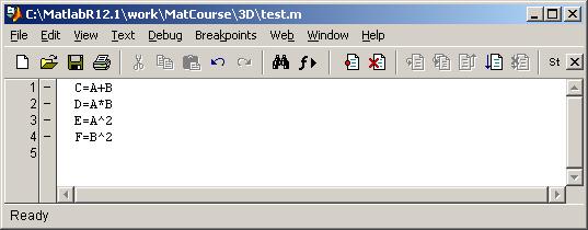
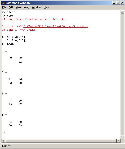
example, consider the following simple script test.m which produces the sum, product and
squares of two matrices A and B.
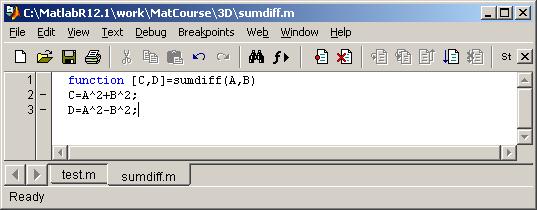
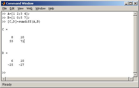
A Matlab function differs from a script in that it accepts an input argument (a group of input variables) and returns a series of output variables. The function format is as follows:
|
Function Body |
where [ O1 O2 . . . Om ] is the set of output variables and [ I1 I2 . . . Ik] the input argument. A function can be called from the command line by typing its name followed by the input argument included in parentheses or from inside a script or another function. Any variable in the function body is local to the function. As an example, consider the following function M-file which accepts two matrices A and B as an input and returns the sum and the difference of their squares.
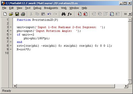
In this illustrative example we exploit basic Matlab matrix operations to describe and eventually execute rigid body motions in two and three dimensions. Rigid bodies are geometrical objects such as tetrahedra, hexahedra, pyramids, prisms, cubes, and spheres. It is well known from analytical geometry that any motion of an object (except reflections) can be decomposed to a sequence of simple geometrical transformations, namely translations and rotations. Moreover, such a transformation is characterized by a matrix. For example, a two dimensional counter clockwise rotation of s degrees around the origin on a plane is achieved by using the matrix
![]()
![]()
Then, if we want to rotate the point (x, y), s degrees around (0, 0) we simply need to multiply R(s) by (x, y); the product is the rotated point.
In a similar fashion, translation by a vector is characterized by the matrix

Also, we may combine these transformations by simply multiplying the corresponding matrices. For instance, the transform first translates the vector, a and b units in the x and y directions respectively and then rotates it by s degrees.
The case of reflections is less complex. As a paradigm, consider reflection of a point (x, y) with respect to the x-axis. Then the image of (x, y) is simply (x, -y). This simple transformation can be represented by the matrix
![]()
These ideas can easily be generalized in three dimensions, which is presented in our example script later in this document. They may also be generalized in higher dimensions, but this is outside of the scope of this introductory material.
The example below executes four kinds of geometrical transformations of a polygon on the plane:
(i)
Rotation with respect to the axis�s origin (0,0)
(iii) Reflection with respect to either the x-axis or the y-axis
(iv) Scaling with respect to a factor m
As mentioned in the introduction, all these transformations are represented by the following matrices:
![]() for case (i)
for case (i)
 for case (ii)
![]() (Reflection with respect to the xx` axis)
(Reflection with respect to the xx` axis)
![]() (Reflection with respect to the yy` axis)
(Reflection with respect to the yy` axis)
![]() for case (iv)
for case (iv)
The transformation matrix is two by two, in all cases but (ii), in which case it is three by three. The reasoning for this exception is that it is impossible to describe a translation on the plane by a two by two matrix (we present the proof in the Appendix for those interested). To overcome this restriction we add to each point of the plane a fictitious coordinate equal to 1. Then (x, y) is represented by (x, y, 1) and the translated point (x+a, y+b) by (x+a, y+b, 1) . Now, we may check th
hence the trick of adding the element 1 to each pair results to a universal matrix describing the translation. In this code we use the representation (x, y, 1) rather than (x, y) for cases (i), (iii), (iv); therefore, we also need to use slightly modified versions of the matrices R(s), Ref, S(m) . That is:
or
and
Program Description
The user provides the number of vertices of the polygon
and their x and y
coordinates. The coordinates are stored in the polygon matrix P, whose columns are the triples [x y
1]. Then the user specifies the kind of transformation desired and the program
calls one of the following functions:
Rotation2D
(for rotation around the axes origin)
Translation2D (for
translation)
Reflection2D (for
reflection with respect to the x or y axes)
Scaling2D
(for uniform scaling by a factor
The transformed polygon is
stored in matrix T in the same way as the initial one is
stored in P. Finally the program
plots the initial and transformed polygons.
All four functions have the same simple structure. The only input variable is the polygon matrix P. The user provides information about scaling factors, rotation angles and any other relevant data and the corresponding transform matrices are constructed. These matrices are then multiplied from the right by P to produce the transformed polygon matrix (R, T, Ref or S), which is returned to the main program.
Our 3D script accommodates both polygonal lines and two
kinds of rigid bodies (tetrahedra and hexahedra), referred to as �objects� in
the sequel. The basic geometrical transformations are again translations,
scaling, reflections (with respect to the
xy, yz, or xz planes) and rotations around arbitrary user-defined axes.
The latter case is relatively complex, however we have included in the code, as
a separate option, rotation of an object with respect to the z
axis (which is a straightforward extension of the 2D rotation around the
origin). As in the 2D case we introduce a fictitious coordinate, equal to one,
to each polygonal lines� or rigid bodies� vertex. Hence, any
point (x, y) is represented as (x, y, 1) .
The 3D transforms� matrices are quite analogous to the
2D ones and are given by:
 (for rotation
around the z-axis by angle s)
(for rotation
around the z-axis by angle s)
 (for
translation a1, b1, c1 units
in the x, y, z directions respectively)
(for
translation a1, b1, c1 units
in the x, y, z directions respectively)
 (for
scaling by a factor m)
(for
scaling by a factor m)
 (for
reflection with respect to the
yz-plane)
(for
reflection with respect to the
yz-plane)
or
 (for
reflection with respect to the
xz-plane)
(for
reflection with respect to the
xz-plane)
or
 (for reflection with respect to the
xy-plane)
(for reflection with respect to the
xy-plane)
The user manually inputs the coordinates of the object�s
vertices, which then are stored in matrix P. The first, second and third rows
of P contain the x,
y and z
coordinates of the vertices respectively. The user may then choose
between a polygonal line or a rigid body. Next, the user selects the desired
transformation, and one of the following functions is called:
zrotation3D (for
rotation of the object around the z-axis)
translation3D (for translation)
scaling3D
(for scaling)
arbrotation3D (for rotation around a user
defined axis)
reflection3D (for reflection
through the xy, yz or xz planes)
Once the function returns the transformed object matrix
T, both the original and transformed objects are graphed. Note that we are using
different plot commands for the objects we are treating (plot3 for polygonal
lines, fill3 for rigid bodies).
The structures of functions reflection3D, scaling3D,
translation3D and zrotation3D are quite similar. As in the 2D case, the only
input variable for each function is the object�s matrix P. The user is asked to
provide the necessary parameter values (e.g, scaling factors, direction shifts)
and the transformation matrix is constructed. Then P is multiplied from the left
with the transformation matrix to produce T, the transformed object�s matrix,
which is returned to the main program.
Section 6:
Simulink and Matlab
Toolboxes Introduction In this section we briefly refer
to Simulink, an application accompanying Matlab, which is frequently used
in Control Engineering problems (particularly in Electrical and Aeronautical
Engineering). We also comment on the Control System & Optimization
toolboxes. A detailed discussion of these topics will be the scope of an
upcoming advanced Matlab tutorial. Simulink Simulink is a simulation tools
library for dynamical systems. Any system in nature can be formally thought of
as a �black box� receiving an input vector u and eliciting a unique
output vector y. If both u and y vary across time, the
system is a dynamic one. Associated with a system is the
so-called state vector which (loosely speaking) contains the required
information at time to that, together with
knowledge of the input for time greater than to ,
uniquely determines the output for t>to . A
general continuous dynamical system can be modeled by using the following set of
ordinary differential and algebraic equations: for t>to and x(to)=xo ,
where f, g are general (possibly non-linear
functions). In the following we will consider only linear systems of the
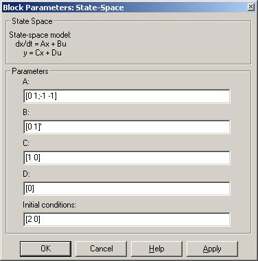
form: where A, B, C, D are matrices and x, u, y the state, input and output vectors
respectively. Of course the dimensions of A, B, C, D are such that the matrix manipulations
on the right hand side of (1) are
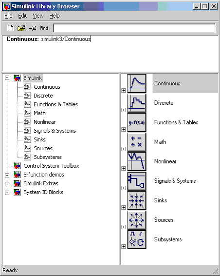
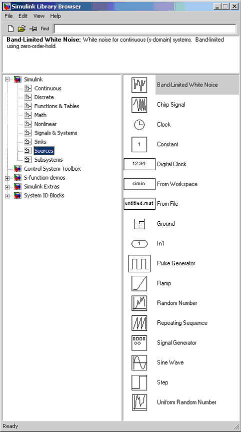
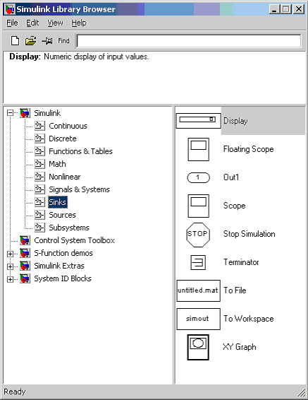
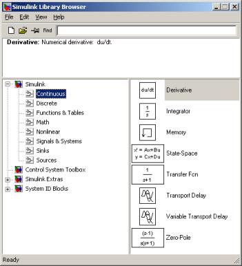
well defined. Simulink Library Browser Simulink can be launched by
double-clicking on the Simulink icon in the Launch pad window of the default
Matlab desktop. The library's functionalities are
divided into eight groups (click on any of the category icons for both the Unix
or Windows versions). For example, the categories Sources and Sinks
contain various kinds of inputs and ways to handle or display the output.
Later in this document, we will also use the group Continuous which deals
with dynamical systems. The images below illustrate the Simulink interface for
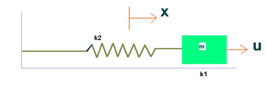
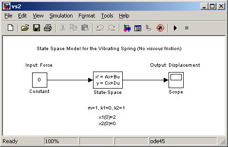
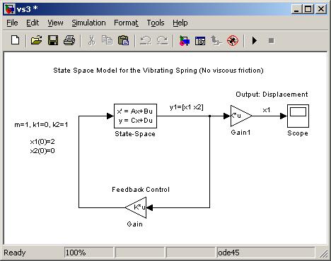
the categories Sources, Sinks, and Continuous. Construction/ Simulation of Dynamical Systems In this section, we consider a simple physical example to
illustrate the usage of Simulink. One of the simplest systems introduced in
mechanics courses is the vibrating spring, which can be modeled by the
ordinary differential equation Here m is
the mass of the body supported by the
spring; k1 and k2 are
the viscous and spring friction coefficients respectively, and u
is the force applied to the body. The unknown function y
is the distance of the body from the equilibrium position. Our first
observation is that the differential equation describing the motion of the body
is of the second order (in other words the highest differentiation order of the
equation is 2). To reduce it to a system of differential equations of the first
order (so that we can use Simulink) we make the following substitution: Then (1) becomes: or in matrix form: Here x1 and x2 are
the state variables and u the input to the system. The output can
be selected in various ways depending on what characteristics of the system are
desired to be measured; it could
be x1 (displacement), x2
(velocity) or a linear combination
of x1, x2, and u. For our
purposes we simply define the output to be x1 . That
is, in matrix form. Equations (3) and
(4) constitute the representation of the system in the form (1), with Furthermore, we take it that that is Our initial conditions
are x1(0)=2, x2(0)=0 , that is, at
time t=0 the body is located at a distance of 2
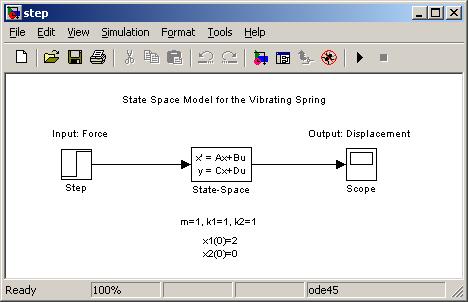
units from the equilibrium position and its velocity is 0. The next step
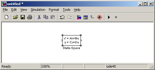
is to build the system using Simulink. Clicking on the New model button
on the upper left corner of the
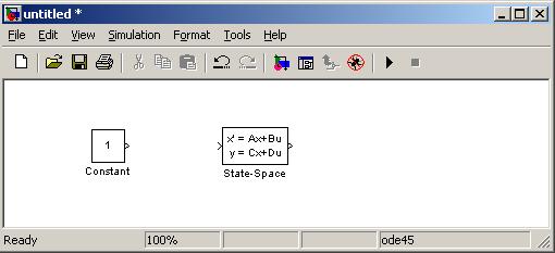
Simulink library browser a window pops out. Next double click on the
Continuous button, select the State-Space icon and drag it into
the new model window. Next, double click the
Sources icon to select an input for the system. In this example we will
choose the input Constant and drag it into the new model window. By
double clicking on the dragged Constant icon, we can specify the value of
the constant input. Here we specify
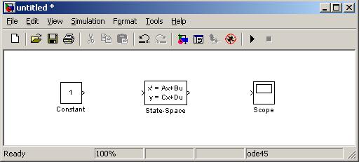
u=1. The output is selected by
clicking on the Sinks button. In this example, we choose Scope
icon (which will provide a graph of the system�s output) and drag the icon into
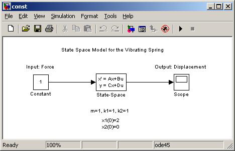
the model window. Next, connect the system blocks
with arrows. For example, to connect the constant and state-space blocks, click
on the right arrow of the constant block and move the cursor to the left arrow
of the state-space block while holding the left mouse key down. We can also add
text on the model window by double clicking at any point of it and inserting the
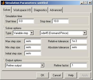
desired information. Finally, select Simulation
-> Simulation Parameters> to specify the simulation parameters (in this
case, we will choose the simulation initial and final time and the ODE solver).
In this example we take it: Now that the system has been
built up, we are ready to run the simulation, which will numerically solve the
system of ODEs to obtain the output
y. Press Start on the Simulation toolbar, then double click
on the Scope icon to obtain a plot of the output. We observe that the displacement
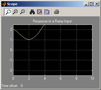
remains constant after approximately t=9. Next we change the system�s input to a
ramp (i.e., a constantly increasing unidirectional force). We specify the ramp
input parameters by double-clicking on the Ramp icon and choosing
slope=1, start time=0 and initial output=0. In the following figures we present
the modified system and its response. As expected, since the force
acting on the body is increasing in magnitude and doesn�t change direction, the
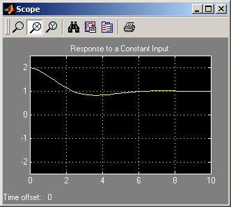
distance from the equilibrium point increases. Next, we consider the case of a
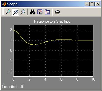
step input (i.e., a force spontaneously changing its magnitude at some time ).
The step function parameters are specified by double-clicking on the Step
icon and choosing step time=1, initial value=0 and final value=1. Below we
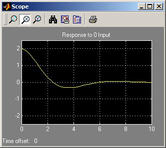
illustrate the input and the graphical output for the step input system. Next, we consider the case of zero force acting on the
body; that is, we have a constant input equal to zero. We expect that the body
will eventually return to the equilibrium
position x1=0 , and indeed this is what our
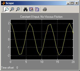
model predicts. In the previous examples (with
the exception of the ramp input), the system�s output eventually approaches a
constant value. Let�s examine the case where viscous friction is negligible
(that is, k1=0 ) and again the input force is
the constant 0 (double click on State-Space icon and adjust A to [0 1; -1
0]). We expect that the body will be
moving internally, since no force exists to counterbalance the spring's force
acting on it. Indeed, the output of the system (displacement of the body)
oscillates between the extreme values
-2 and 2. In our last example we try to
correct this behavior and make the system�s output approach the value 0 (that
is, to make the body return to the equilibrium position) by introducing a
so-called feedback control law. More precisely, we define a new input to the
system which is not user supported as in the previous examples, but depends on
the system�s output. In other words, the system�s output simultaneously defines
its input. We define: Given our choice of K, our system becomes: but using Simulink we actually
develop the equivalent
formulation To construct this model drag the
Gain blocks from the Math library (and again double click on them
to specify the gain matrices). Also, in order to rotate a Gain block
simply right-click on it, choose the Format option from the pull-down
menu that appears and then select the options Rotate block or Flip
block. In the next two figures the feedback-controlled system is presented
along with its output. By adding the feedback control,
the body returns to its equilibrium position. The Control System Toolbox
contains routines for the design, manipulation and optimization of LTI (linear
time invariant) systems (systems of the form (1) in the Simulink section, where
matrices A, B, C, D are constant). It can be used individually or as a
post-processing tool for a system created with Simulink. The Control System
Toolbox also supports two auxiliary applications, the LTI Viewer and the SISO
Design Tool. The LTI Viewer is used to plot graphs of the system response due to
various inputs, and the SISO Design Tool is used to design single
input-single output systems, that is systems for which the input and output
vectors have dimensions 1 by 1. These applications can be launched by
double-clicking on the Control System Toolbox icon in the Launch Pad window of
the default Matlab desktop. We don�t commend on the SISO design tool, since that
would require knowledge of control theory, but we give an example of the use of
LTI Viewer. Consider once more the system we used in the Simulink examples, that
is To import the system to the LTI
Viewer, we create a system object using the ss command. Below, we
designate our system as an object called s1. >>
A=[0 1;-1 -1]; x1 x2 b
= u1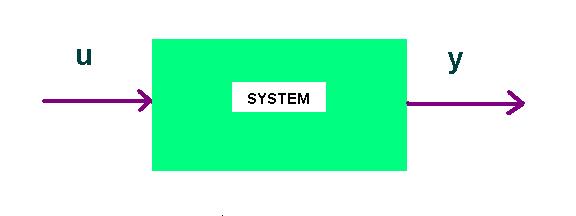
![]()
![]() (1)
(1)
![]() (2)
(2) ![]()
 (3)
(3) (4)
(4)  ,
,
 ,
, ![]() ,
,
![]() .
.![]()
![]()
![]()


![]()

Control System Toolbox
 ,
, ![]()
![]() ,
, ![]()
>> B=[0 1]';
>> C=[1
0];
>> D=0;
>> s1=ss(A,B,C,D)
x1 0 1
x2
-1 -1
x1 0
x2 1
c
=
x1 x2
y1 1 0
u1
y1 0
Continuous-time
model.
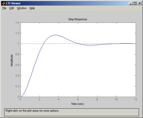
Next, select the options New Viewer and Import from the File menu, and then choose the object s1. The following figure will appear, showing the response of the system to a unit step input. By default the initial condition here is zero.
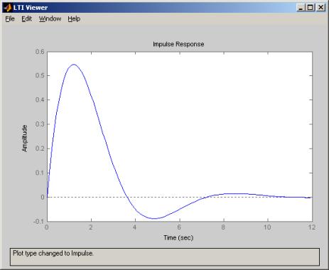
Next, right click on that figure, and select Plot type option and then the Impulse option. The resulting figure is a plot of the response of the system to a unit impulse at time zero.
Optimization Toolbox
The Optimization Toolbox offers a rich variety of routines used for the minimization and maximization of functions under constraints. We will describe only two simple and commonly used examples. The first one is fminbnd which calculates the location in a given interval at which a function attains its minimum. Note that the maximum of a function f(x) is equal to minus the minimum of -f(x) , hence we can use fminbnd to compute locations of maxima of functions too. Suppose now that we want to compute the minimum and maximum values of f(x) = x e-x 2 in the interval [-1, 1] .
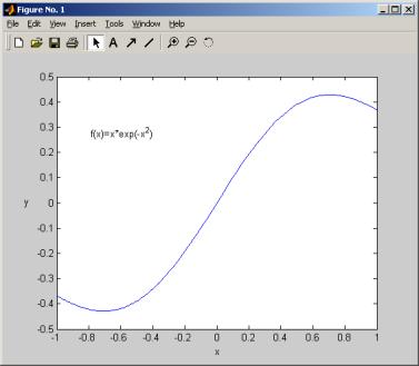
Then we type in the command
line:
>> x=fminbnd('x*exp(-x^2)',-1,1)
x =
-0.7071
>> x*exp(-x^2)
ans =
-0.4289
>> x=fminbnd('-x*exp(-x^2)',-1,1)
x =
0.7071
>> -(-x*exp(-x^2))
ans =
0.4289
The minimum and maximum values of f(x) = x e-x 2 are -0.4289 and 0.4289 and are attained at -0.7071 and 0.7071 respectively. Next, consider the problem of linear optimization, which is frequently encountered in Operations Research and Mathematical Economy. The objective is to find n real numbers that minimize the linear expression
![]()
subject to the constraints:
or in matrix form,
minimize
![]()
such that
![]()
The problem can be solved via the function linprog . As an example consider the following 2-D linear optimization problem:
Minimize
![]()
so that the constraints
![]()
![]()
![]()
![]()
hold.
To solve it we type:
>>
c=[2 3];
>> A=[-3 4; 3 1; 1 -2; -2 -1];
>> b=[0 15 5 0]';
>> linprog(c,A,b)
Optimization terminated successfully.
ans
=
1.0000
-2.0000
Next we give a geometrical interpretation of this solution. It can be shown that the pair that solves the problem, is one of the vertices of the quadrilateral in the following figure:
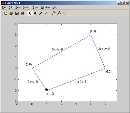
The edges of the trapezoid correspond to the optimization constraints and the points in its interior satisfy all of them, hence the solution must be attained in the trapezoid or on its boundary. Due to a theorem in Linear Optimization, the solution is attained at one of the trapezoids� vertices, in this case at the point (1,-2).
Appendix ![]()
![]()
For all x and y, real numbers. Then carrying out the matrix manipulations we have
![]()
and equating the vector components we get the following two equations:
![]()
Manipulating these expressions we end up with
for all real x and y (since the transformation should be generic, that is valid for all real x, y); therefore, all coefficients in the latter equations must be zero, which implies
![]()
This is a contradiction, since (a, b) is different from (0, 0).