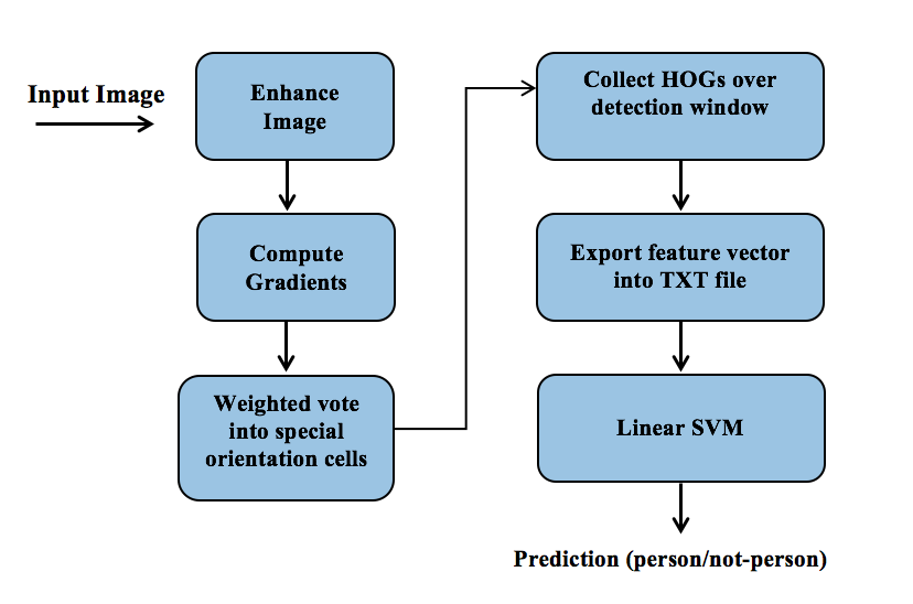
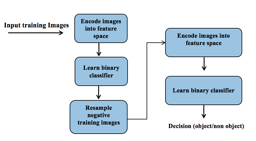
Pedestrians Detection
HOG based Implementation
We used a part of the data set of INRIA Person Dataset.
The part we used is:
| Positive | Negative | |
| Training | jdjdj96x160H96/Train/pos | jdjdjTrain/neg |
| Testing | jdjdj70X134H96/Test/pos | jdjdjTest/neg |
Some notes:
Positive images: For training we used 2416 images of size 69x160. For testing we used 1126 images of size 70x134.
Negative images : For training we used a fixed set of 12180 patches sampled randomly from 1218 training images. And tested on 4530 patches sampled randomly from 453 person-free testing images.
* Negative means no humans in it.
Examples for negative/positive images:
Train positive:
 |
 |
 |
 |
 |
 |
 |
 |
Test positive:
 |
 |
 |
   |
 |
 |
 |
   |
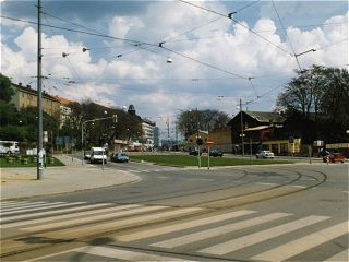
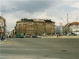
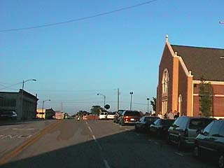
Train negative:
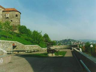 |
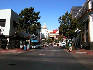 |
 |
 |
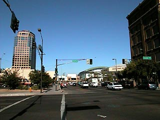
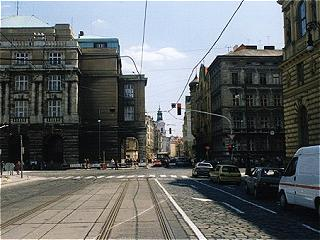
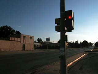
Test negative:
 |
 |
 |
 |
How we used this data?
Positives:
As one can see in the examples above, in the positive images, a human is centred in the middle.
In training\testing phase for positive images, we centered the 90x160\70x134 images and then extracted the features from it.
Negatives:
In negative images, we cropped the images by taking randomly 10 patches from each image.
The cropped images is of size 63x126.
- The MATLAB functions that are responsible for training and testing are testTrain_dataNeg.m and testTrain_dataPos.m. Both functions take as parameters the type of the classifier (SVM, NN) and a flag that says if its testing or training mode (1 for training positive and -1 for traing negatives and 0 for testing).
Feature Extraction: Histogram of Oriented Gradients (HOG)
We do feature extraction on windows (images) of size 63x126, this choice was made because according to the paper the block size is 18x18 pixels which is constructed from 3x3 cells and every cell is 6x6 pixels.
In the paper they tested a various block sizes (2x2 per block 1x1 per block..) and different cell size (12x12, 10x10, 8x8 pixels), then they figured that 6x6 pixels cell size and 3x3 cells per block gave the best results, and it seems that this cell size is the same as the size of the human limp. The window size suggested in the paper was 64x128.
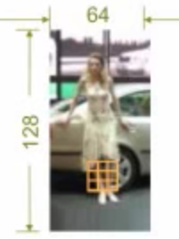
* We took 63x126 window size because we wanted to divide the image into blocks with overlapping 50%, since 63 and 126 can be divided by 9.
HOG descriptors:
Given a 63x126 image (window), we extract the feature vector from it following these steps:
- Compute image gradients both for X and Y using [-1,0,1] mask. We tried computing the gradients by the MATLAB function imgradient which uses sobel mask as default, but it did not give us results as good as the [-1,0,1] mask.
- Next we want to compute the magnitude and the orientation of the gradients. Let
 be the image gradients (Jx= X-Gradient and Jy =Y-Gradient). Now we can compute the gradient magnitude using this formula:
  , and we can compute the edges orientation using this formula:
  .
. - Orientations must be values from 0-180° “unsigned” gradient, and since tan-1 gives us values between -90° and 90° we added 180 to the negative results from the formula above
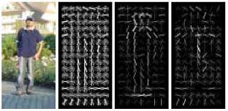
- We create 9 bins, where each bin is the gradient orientation between 0-20, 20-40 and so on till 160-180. This way each pixel calculates a weighted vote for an edge orientation histogram channel based on the orientation of the gradient element centred on it.
- Now we collect HOGs: looping over the image blocks and calculate the HOG vector for each block (overlapping 50% between each block).
- How do we collect HOGs ? We take in every iteration a block of size 18x18 and get it's magnitude and orientations bins from what we calculated ealier.
- We divide the 18x18 block into 3x3 cells and for every cell we allocate 9 places in the hog vector, where every place says sums of the magnitude of that pixels in that cell which their orientation between 0°-20°, and between 20°-40° and so on till 160º-180º. We have these values we calculated them in previous steps.
- For every cell in the block we do this and we get 81 slots for every block in the HOGs vector.
- We normalise every block HOGs vector using this formula:
 where v is 81x1 sized block-hog vector. (the normalisation step was necessary to get rid of the changing of the light).
 - At the end we get a HOGs vector for the whole 63x126 window. This vector size is 81*78=6318 (78 is the number of the block in each window, since we have 50% overlapping between blocks, and block size is 18x18).
Summery:
We take a window image of size 63x126, calculate it's gradients (X-gradient and Y-gradient), after that we calculate for each pixel it's weighted vote for an edge orientation histogram channel based on the orientation of the gradient element centred on it, and the votes are accumulated into orientation bins over local spatial regions (cell). The orientation bins are evenly spaced over 0°– 180° (“unsigned” gradient). The vote is a function of the gradient magnitude at the pixel representing soft presence/absence of an edge at the pixel. (based on the paper). In other words. in each cell in the block we take the pixel indensity (orientation and magnitude), and we create a Histogram of Orientation of the cell and read the histogram by the Magnitude of the gradient.
This process creates a vector of Histogram of Orientations Gradients and it represents our feature vector.
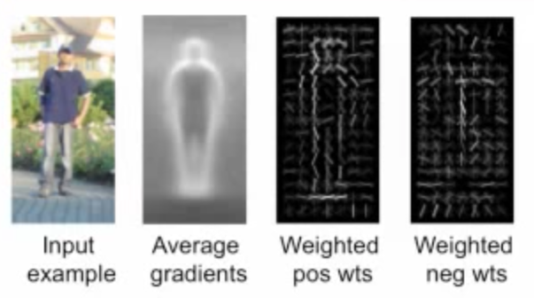
- Each line in the Weighted images here (pos and neg) respondes to the cell and the dominant orientation in that cell and the magnitude of the line is equal to the magnitude of the weight.
Note: This proccess is done in MATLAB file findHogs.m, where this function returns as an argument a features vector of size 6318.
Learning/Training Phase (SVM):
After calculating the features vectors, it is time to train our classifier.
Recalling the training images we talked about in previous section, we had positive samples and negative samples for training.
Training for positives:
As we said earlier, the positive images for training are of size 96x160. Our feature extractor expects a 63x126 image, so before we send the image to the feature extractor (findHogs.m), we center the image (taking the middle 63x126 pixels) and send in to the function.
The training for positives is being done in MATLAB function testTrain_dataPos(classifier,trainTest). The classifier parameter stands for the type of the classifier (SVM or NN), and trainTest parameter stands for the mode, in our case now we called for training positive testTrain_dataPos('SVM',1);
This function will ask to load all the images you would like to train (all in once), and then loop over all these images and calculates the HOGs vector for each one.
After calculating the HOGs vector we call a function export_features_SVM(features_vec,target) that exports the HOGs vector into a txt file that will be send to the SVM classifier holding all the features vectors. (the target parameter is a flag for testing or training)
The txt content format is as follows:
<target> <feature>:<value> <feature>:<value> ... <feature>:<value>
where <target> .=. +1 | -1 | 0 | --> +1 for positive trainig mode, -1 for negative training mode, 0 is for unknown which is test mode.
Examples:
1 1:0.233 2:0.312 3:0.432 --> target=1 (training postive mode), 3 features separeted by space charecher
-1 1:0.2782 2:0.293 3:0.9281 4:0.152 --> target=-1 (training negative mode), 4 features.
0 1:0.235 2:0.322 3:0.442 --> target=0 (test case), 3 features.
Training for negatives:
As we said in the previus section, the 1218 negative images have different sizes. We said also that we would train 12180 negative image.
How do we use this data for training?
The training for negatives is being done in MATLAB function testTrain_dataNeg(classifier,trainTest). This function loads all the 1218 images, and cut randomly 10 patches of size 63x126 from each image, giving us 12180 negative images of size 63x126 for training. We called the function with therse parameters: testTrain_dataNeg('SVM',-1)
Now as we did with the positive training, we calculate the features vector for every negative image and then save it into the txt file we used in positive training. The txt file name is trainingData.txt.
Train?
After we calculated all the features vectors for both negative and positive samples and saves them in a txt file we want to train the classifier over these feature vectors.
We used SVMLight as our classifier in this project. The SVM we used is implemented by Thorsten Joachims and can be found in this link. The implementation is in C.
Some of the program's features:
Fast optimization algorithm- working set selection based on steepest feasible descent
- "shrinking" heuristic
- caching of kernel evaluations
- use of folding in the linear case
- solves classification and regression problems. For multivariate and structured outputs use SVMstruct.
- includes algorithm for approximately training large transductive SVMs (TSVMs).
- can train SVMs with cost models and example dependent costs.
- and more..
To train the classifier we call svm_learn with these parameters: example_file and model_file. The input file example_file contains the training examples which we saved as txt file in the above steps. The result of svm_learn is the model which is learned from the training data in example_file. The model is written to model_file.
- We called the svm_learn from MATLAB with these parameters: system('svm_learn trainingData.txt model.txt');
- Now we have our own model.txt for our training data which can be used to classify the unknown samples.
Testing Phase (SVM):
To test our classifier, as we explained in the previous section we use 1126 positive images of size 70x134 and as in training we center these images and take the middle 63x126 pixels. And we use 453 negative images of different sizes and as in training we cropped randomly 10 patches from each image giving us 4530 negative images for testing.
We follow the steps as in training, we call testTrain_dataPos('SVM',0) for positives and testTrain_dataNeg('SVM',0) for negatives.
We get two files to test, one that holds the negative samples (testNeg.txt) and the other one for positive samples (testPos.txt).
To test these two files we call svm_classify with the parameters example_file, model_file and output_file. example_file is the txt file that contains the features vectors (neg/pos), model_file is the model.txt file that we trained in the previous section. output_file is the prediction result, a negative or positive value for each line, the sign of this value determines the predicted class.
- We called the svm_classify twice from MATLAB with these parameters:
- For positive samples:system('svm_classify testPos.txt model.txt predPos.txt');
- For negative samples: system('svm_classify testNeg.txt model.txt predNeg.txt');
- Now we have two predictions files, one for negatives (predNeg.txt) and one for the positives (predPos.txt).
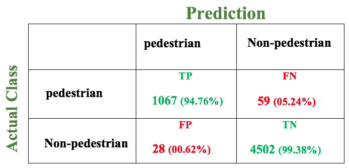
Testing Results:
Positive: recall, we tested 1126 positive windows. We took the predPos.txt and checked the values (positive values means that the window (63x126 image) in that line has a pedestrian, else, if it is negative value, it means that there is no pedestrian in that window.
Negative: recall, we tested 4530 negative windows. We took the predNeg.txt and checked the values as in positive case.
The results are:

Testing In Real World:
After training and testing our features, which gave us a satisfying results of percision and accuracy, now we are ready to test our program in the real world.
We took a couple of random images from real world streets and tested on them.
Here are some of the results:
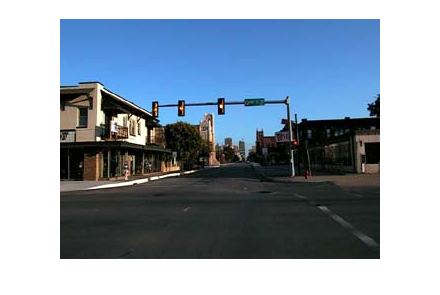
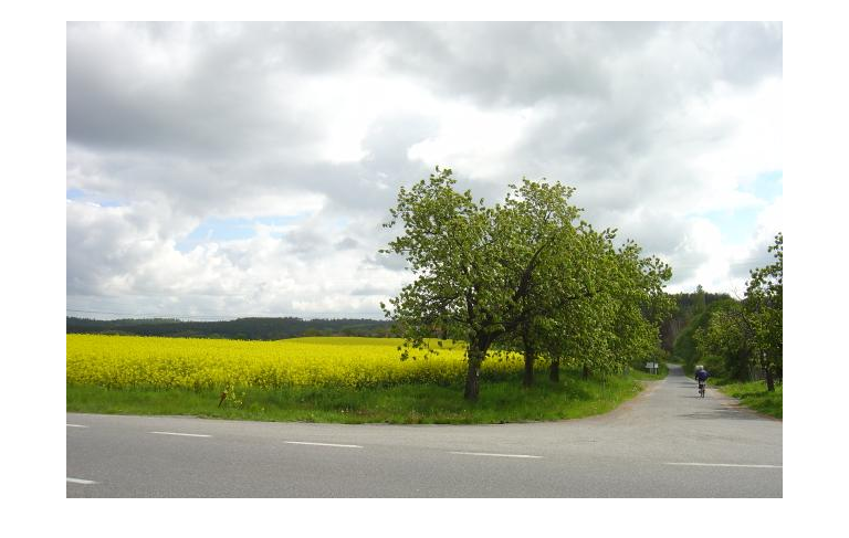
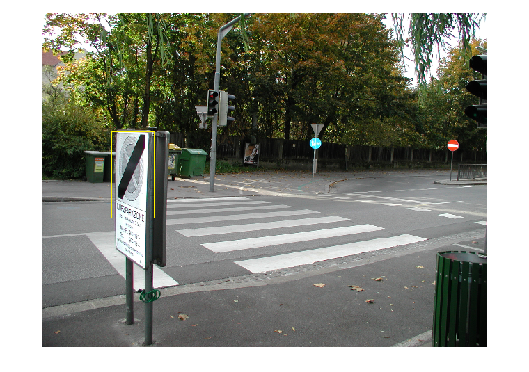
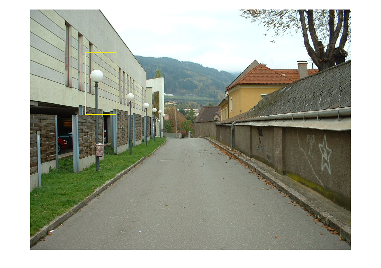
Taking negative images (no pedestrians on it), we got these results:
A 100% accurcy, no misses: (note: we resized some images here to fit the screen)
One Miss: (no resize for images here)
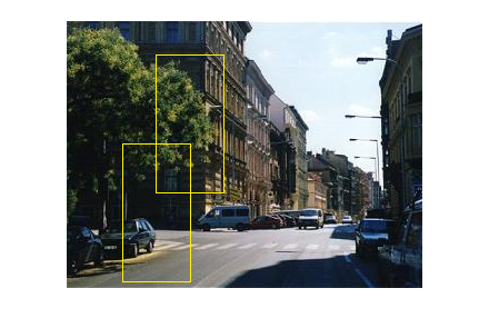
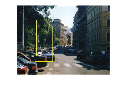
Other Results:
How do we test Real World Images?:
- We take the image (of unknows size, and unknows content).
- We divide this image into windows of size 63x126 with 10 pixels overlapping difference between every two consecutive windows, in horizontal and vertical direction.
- Extract features per every window.
- Classify every window (send the vector to the SVM classifier).
- Highlight every positive window (positives values returned by the classifier).
Important NOTE:
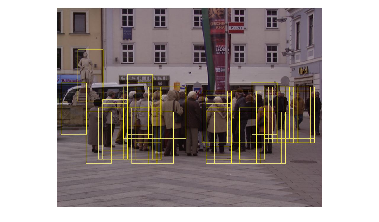
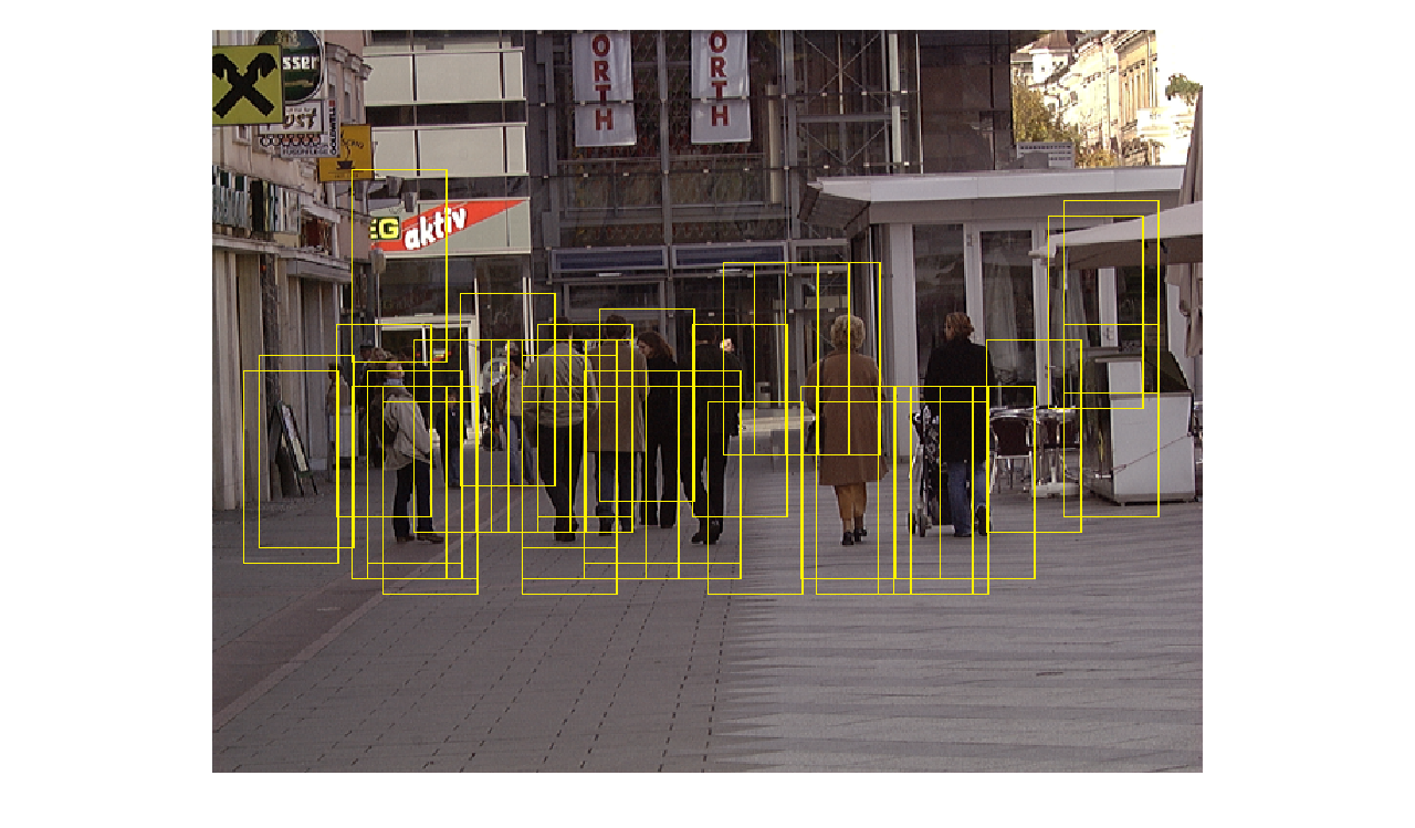
Beacuase of the fact that we take overlapping windows in the image, we might detect the same pedestrian more than once.
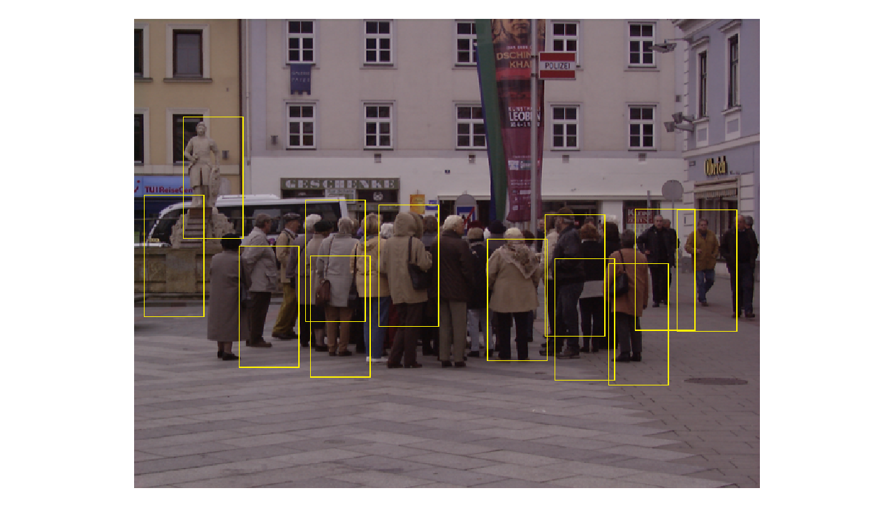
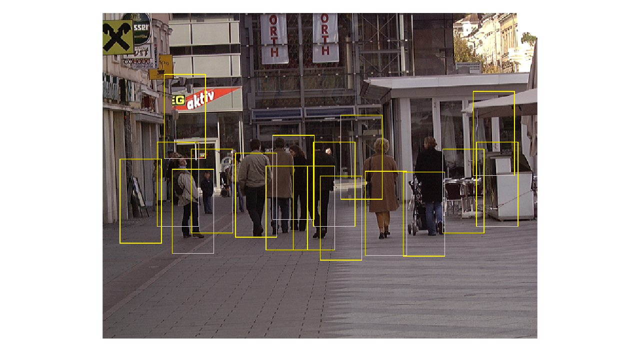
To solve this issue and to get rid of the redandent highlights for the same pedestrian, we did Mean Shift Cluster Algorithm over the positive windows.
We will explain the method of Clustring in the next section, now we will just show the results before and after using the mean shift algorithm.
Here are some results of Positive images:
* This image is the result BEFORE applying the Mean Shift Algorithm:
* This image is the result AFTER applying the Mean Shift Algorithm:
- Here is another example of the efficiency of this MS Algorithm step:
After Mean Shift:
More results:
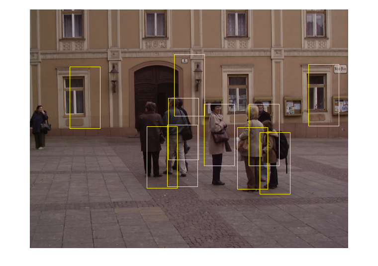
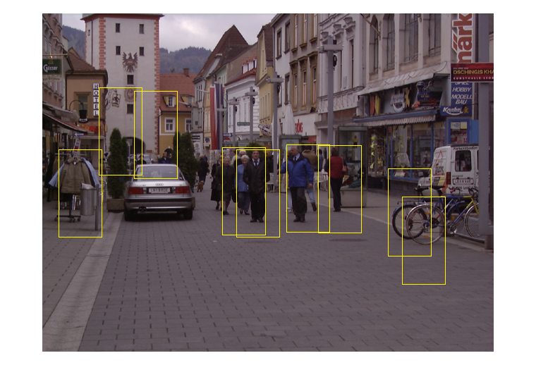
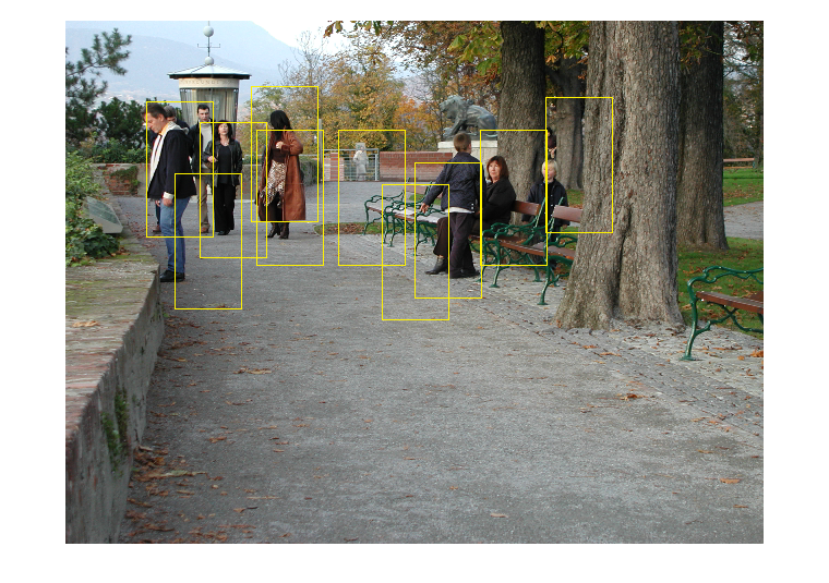
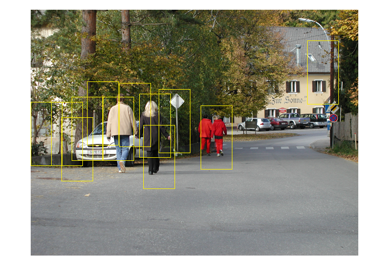
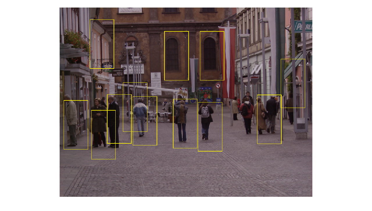
As we mentioned earlier, we used 10 pixels overlapping difference between every two consecutive windows, in horizontal and vertical direction (that means, we enabled overlapping for all except of 10 pixels between).
Because of that, we found redundancy when detecting the same pedestrian, and more than one window for the same pedestrian. So we had to use a clustering algorithm, and since we don't know the number of pedestrians that are supposed to be detected, none the less we have no idea of how many clusters of windows we need, we had to use the mean-shift algorithm, a clustering method that doesn't require prior knowledge of the number of clusters.
The function meanShift.m receives two inputs: The first input is a matrix that contains two rows and number of columns equals to the number of the detected positive windows. The first row contains the first dimensions of the upper-left corner of the windows, and the second row contains the second dimensions of the upper-left corner of the windows. Therefore, for each column, there's the location of the upper-left corner of the related window. The second input is the radius, we used it to set the maximum expected radius between clusters and the original points.
We have to mention that we implemented a limited version of mean-shift algorithm, that works only for our need, and supports only two-dimensional points.
After applying the mean-shift function, the output should be a matrix (as the same as the input), but with columns that have the locations (two dimensions) of the clusters.
- SVMLight : SVMLight Support Vector Machine.
- The related paper: Histograms of Oriented Gradients for Human Detection
- The Data Set: INRIA Person Dataset.
Related MATLAB Files:
Pedestrian_Detetction_MATLAB.zip
Trained Data (model.txt file produced by the svm_learn in the learning phase)
Notes:
- The zip file contains all the matlab functions we used in our project.
- One of the files is main.m which contains instructions on how you can use the program.
- In order to be able to use the program you have to download the svm_classify excusable from the link above.
- We already did the training phase, you do not have to do it again (it takes a little bit time), so in order to use the svm_classify you need to download the model.txt file.
Credits:
This project was prepared by Ezza Abu Elheja and Mustafa Mahameed, students at the department of Computer Science at the University Of Haifa as a project in the course Computer Vision supervised by Prof. Daniel Kerel.
