Double declining is type of acceleration depreciation method. Accelerated depreciation means it recognizes a higher depreciation at the beginning of the life time of the asset. First let’s understand what declining appreciation is ?. Double declining depreciation value is twice the value of the straight line depreciation. In double declining previous years asset value becomes the input to the next year’s depreciation calculation. Below figure ‘Double declining balance’ shows how calculations are done for every year. The basic formula for calculating depreciation is as below.
Depreciation expense = previous period value * ( Factor / Life of Asset )
From the above formula we will get depreciation expense on a per month basis. Previous period value is the value of the asset after deducting the depreciation of that year. Factor value is two for double declining depreciation. Life of asset is the life of the asset.
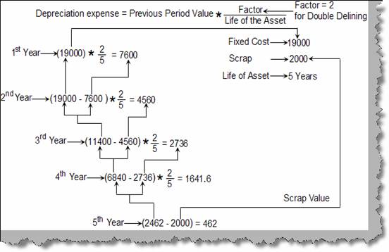
So let’s analyze the below calculation for double declining balance. In the below example we have asset of cost around 19000 with scrap value of 2000 and life of the asset is five years. So the first year of calculation is fixed cost multiplied by factor divided by life of asset which comes to around 7600. Now to calculate for the second year we subtract the depreciation of the first year from the fixed cost and multiple by factor divided by life of asset. In the same way we carry forward for third and fourth year. Now for the fifth year we deduct the previous brought forward from the scrap value, because this is the final year of the life of asset. So for the final year the depreciation is 462. Try to follow the way carry forwards are taken from previous year to the next year this will clear your fundamentals in a more appropriate manner.
Figure: - Double declining balance
Ok, the above calculation was very tedious. Excel has provided an easy way i.e. by using ‘DDB’ formula. Below figure ‘DDB in action’ shows how the formula does the calculation. It takes five parameters. We have out arrows to the parameter to understand the same in more visual format.
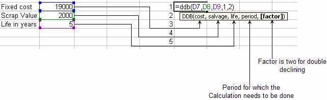
Figure: - DDB in action
1