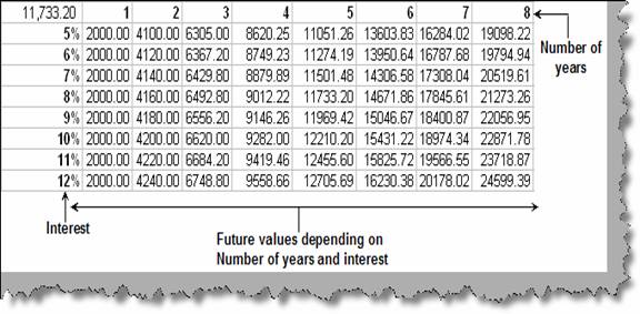
Consider the scenario below as shown in figure ‘Two input view’ where we want to have an overall picture of what will be the return on various values of interest and period.
Figure: - Two input view
The above complex view can be achieved by using ‘Datatables’ in excel. A Data Table will give a view of how by changing certain values in your formulas you can affect the result of your formula. Data Tables can store the results of many different scenarios for you in one table, so that you can analyze them to select which scenario is optimum.
‘Datatables’ can take one input or two inputs. The above figure has two inputs ‘Interest’ and ‘Period (Number of years)’.
So let understand both the ways of analyzing data i.e. ‘Single input’ way and ‘Two input’ way. Let’s take a small sample which calculates future value as shown in figure ‘Single Input Scenario’. So with an initial amount of 2000 invested for 5 years with 8% interest we will get 11733.20 after 5 years. We have found the same by using ‘FV’ formula. If you want to understand ‘FV’ in more detail please refer previous questions.
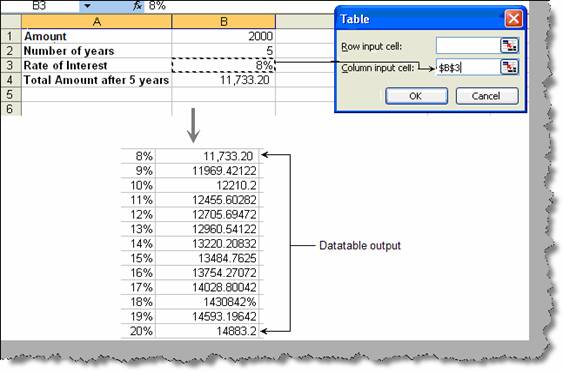
Figure: - Single input scenario
Now we need to find out that with different rate of interest what will be the ‘FV’ i.e. Future value. In the same figure ‘Single input scenario’ we have entered rows from 8% to 20%. In the first row i.e. for 8% we have referenced the column where we have the ‘FV’ formula. This is a very important step if you miss it you will not get proper results. For this scenario the input is the ‘rate of interest’ and we need to find out how much will be the future value after 5 years. In short there is only one input.
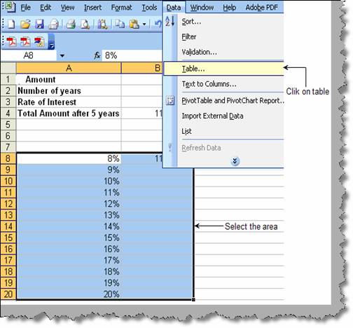
Figure: - Select Area for single input
So the first thing we do is select the area as shown in figure ‘Select area for single input’ and click on data à table. Yu will be then popped with dialog box as shown in figure ‘Dialog box for single input’. The dialog box has two parameters one is the row input cell and the other is the column input cell. Currently we have only one input i.e. ‘Rate of interest’. We do not have a second input currently. So we need to only enter the cell reference of ‘Rate of interest’ in the column input cell of the table dialog box. Once done click and VOILA. You can see the output shown in the same figure for the rate of interest for 5 years period.
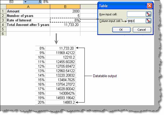
Figure: - Dialog box for single input
Now we add a bit of twist, we add one more input. In other words we add one more input period (number of years). So for various range of interest and period what is the future value.
So as said previously we have two inputs one is the rate of interest and the other is period. In the below figure ‘Two input situation’ we have entered years row wise (1, 2, 3,4,5,6 and 7) and percentage column wise (4% to 17%). Again we have referred the ‘FV’ formula on the row where period is present. This is again a very important step. The position where the reference is done is also important.
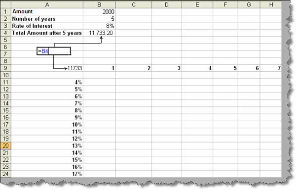
Figure: - Two input situation
Now we select the area we want to the result and click data à table.
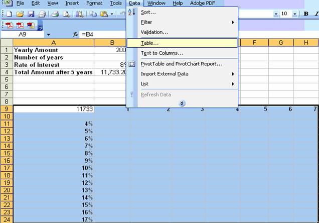
Figure :- Select area for two inputs
We are then popped up with a table dialog box as shown in figure ‘Dialog box popup for two inputs’. We have two inputs one is the column input i.e. rate of interest and second is the row input i.e. number of years. Now click ok and VOILA. You can see how EXCEL has calculated the future value for every combination of interest and period. We have also shown the output in the same figure ‘Dialog box popup for two inputs’.
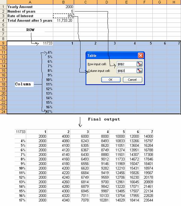
Figure :- Dialog box popup for two inputs