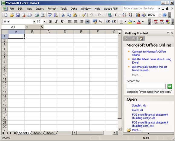
| Getting Familiar with Microsoft Excel This course teaches Microsoft Excel basics. Although knowledge of how to navigate in a Windows environment is helpful, this course was created for the computer novice. To begin, open Microsoft Excel. The screen shown here will appear.
The Title Bar
This lesson will familiarize you with the Microsoft Excel screen. We will start with the Title bar, which is located at the very top of the screen. On the Title bar, Microsoft Excel displays the name of the workbook you are currently using. At the top of your screen, you should see "Microsoft Excel - Book1" or a similar name. The Menu Bar
The Menu bar is directly below the Title bar and displays the menu. The menu begins with the word File and continues with the following: Edit, View, Insert, Format, Tools, Data, Window, and Help. You use the menu to give instructions to the software. Point with your mouse to a menu option and click the left mouse button. A drop-down menu will appear. You can now use the left and right arrow keys on your keyboard to move left and right across the Menu bar options. You can use the up and down arrow keys to move up and down the drop-down menu. To select an option, highlight the item on the drop-down menu and press Enter. An ellipse after a menu item signifies additional options; if you select that option, a dialog box will appear. Toolbars
The Formatting Toolbar Toolbars provide shortcuts to menu commands. Toolbars are generally located just below the Menu bar. Before proceeding with the lesson, make sure the toolbars we will use -- Standard and Formatting -- are available. Worksheets
Microsoft Excel consists of worksheets. Each worksheet contains columns and rows. The columns are lettered A to IV; the rows are numbered 1 to 65536. The combination of column and row coordinates make up a cell address. For example, the cell located in the upper left corner of the worksheet is cell A1, meaning column A, row 1. Cell E10 is located under column E on row 10. You enter your data into the cells on the worksheet. The Formula Bar
If the Formula bar is turned on, the cell address displays on the left side of the Formula bar. Cell entries display on the right side of the Formula bar. Before proceeding, make sure the Formula bar is turned on. The Status Bar
If the Status bar is turned on, it appears at the very bottom of the screen. Before proceeding, make sure the Status bar is turned on. Notice the word "Ready" on the Status bar at the lower left side of the screen. The word "Ready" tells you that Excel is in the Ready mode and awaiting your next command. Other indicators appear on the Status bar in the lower right corner of the screen. Here are some examples: The Num Lock key is a toggle key. Pressing it turns the numeric keypad on and off. You can use the numeric keypad to enter numbers as if you were using a calculator. The letters "NUM" on the Status bar in the lower right corner of the screen indicate that the numeric keypad is on. Other functions that appear on the Status bar are Scroll Lock and End. Scroll Lock and End are also toggle keys. Pressing the key toggles the function between on and off. Scroll Lock causes the pointer movement key to move the window but not the cell pointer. End allows you to jump around the screen. We will discuss both of these later in more detail. Make sure the Scroll Lock and End indicators are off and complete the following exercises. The Down Arrow Key: You can use the down arrow key to move downward on the screen one cell at a time. The Up Arrow Key: You can use the Up Arrow key to move upward on the screen one cell at a time. The Right and Left Arrow Keys: You can use the right and left arrow keys to move right or left one cell at a time. Page Up and Page Down: The Page Up and Page Down keys move the cursor up and down one page at a time. The End Key
The End key, used in conjunction with the arrow keys, causes the cursor to move to the far end of the spreadsheet in the direction of the arrow. Note: If you have entered data into the worksheet, the End key moves you to the end of the data area. The Home Key: The Home key, used in conjunction with the End key, moves you to cell A1 -- or to the beginning of the data area if you have entered data. Scroll Lock
Scroll Lock moves the window, but not the cell pointer. Selecting Cells
If you wish to perform a function on a group of cells, you must first select those cells by highlighting them. Alternative Method - Selecting Cells by Dragging You can also highlight an area by holding down the left mouse button and dragging the mouse over the area. In addition, you can select noncontiguous areas of the worksheet. Closing Microsoft Excel File on menu bar > exit. Entering Text To begin, open Microsoft Excel. For this lesson, your default font should be set to Arial. Let's check to make sure it is. Click on Format, which is located on the Menu bar. > Press the down arrow key until Style is highlighted. > Press Enter. A dialog box will appear. > Click on Modify. > Click on the Font tab, if it is not in the front. > Click on Arial in the Font box, if Arial is not already selected. > Click on OK. > Click again on OK. This lesson will teach you how to enter data into your worksheet. First you place the cursor in the cell in which you would like to enter data, type the data, and then press Enter. Place the cursor in cell A1. > Type John Jordan . Note that the word Ready on the Status bar changes to Enter. > The Backspace key erases one character at a time. Erase " Jordan " by pressing the backspace key until Jordan is erased. > Press Enter. The name "John" should appear in cell A1.
Editing a Cell After you enter data into a cell, you can edit it by pressing F2 while you are in the cell you wish to edit.
Alternate Method Editing a Cell by Using the Formula Bar You can also edit the cell by using the Formula bar. You can change "Jones" to "Joker" by click at the formula bar then backspace to delete what you don't want, then type in. Alternate Method Editing a Cell by Double-Clicking in the Cell You can change "Joker" to "Johnson" by double click at a cell, then make change. Changing a Cell Entry Typing in a cell while you are in the Ready mode will replace the old cell entry with the new information you type. Adjusting the Standard Column Width When you enter Microsoft Excel, the width of each cell is set to a default width. This width is called the standard column width. We need to change the standard column width to complete our exercises. To make the change, follow these steps: Click on Format, which is located on the Menu bar. > Press the down arrow key until Column is highlighted. > Press Enter. > Press the down arrow key until Standard Width is highlighted. > Press Enter. > Type 25 in the Standard Column Width field. > Click on OK. The width of every cell on the worksheet should now be set to 25. Cell Alignment Look at cell A1. The name "Cathy" is aligned with the left side of the cell. You can change the cell alignment.
Centering by Using the Menu To center the name Cathy, follow these steps: Move the cursor to cell A1. > Click on Format, which is located on the Menu bar. > Press the down arrow key until Cells is highlighted. > Press Enter. > Click on the Alignment tab, if it is not in the front. > Click to open the drop-down box associated with the Horizontal field. After the drop-down box is opened, click on Center. > Click on OK to close the dialog box. The name "Cathy" should now be centered.
Right-Aligning by Using the Menu To right-align the name "Cathy," follow these steps: Move the cursor to cell A1. > Click on Format, which is located on the Menu bar. > Press the down arrow key until Cells is highlighted. > Press Enter. > Click on the Alignment tab, if it is not in the front. > Click to open the drop-down box associated with the Horizontal field. After the drop-down box is opened, click on Right. > Click on OK to close the dialog box. The name "Cathy" should now be right-aligned.
Left-Aligning by Using the Menu To left-align the name "Cathy," follow these steps: Move the cursor to cell A1. > Click on Format, which is located on the Menu bar. > Press the down arrow key until Cells is highlighted. > Press Enter. > Click on the alignment tab, if it is not in the front. > Click to open the drop-down box associated with the Horizontal field. After the drop-down box is opened, click on Left (Indent). > Click on OK to close the dialog box. The name "Cathy" should now be left-aligned.
Alternate Method -- Alignment by Using the Formatting Toolbar Using the Formatting toolbar, you can quickly perform functions. You can use the Formatting toolbar to change alignment. Centering by Using the Toolbar To center the name "Cathy," follow these steps: Move the cursor to cell A1. > Click on the Center icon, which is located on the Formatting toolbar.
Right-Aligning by Using the Toolbar To right-align the name "Cathy," follow these steps: Move the cursor to cell A1. > Click on the Align Right icon, which is located on the Formatting toolbar.
Left-Aligning by Using the Toolbar To left-align the name "Cathy," follow these steps: Move the cursor to cell A1. > Click on the Align Left icon, which is located on the Formatting toolbar.
Adding Bold, Underline, and Italic You can bold, underline, or italicize text in Microsoft Excel. You can also combine these features -- in other words, you can bold, underline, and italicize a single piece of text. In the exercises that follow, you will learn three different methods for bolding, italicizing, or underlining text in Microsoft Excel. You will learn to bold, italicize, and underline by using the menu, the icons, and the shortcut keys. Adding Bold -Using the Menu Type Bold in cell A2. Click on the checkmark located on the Formula bar. Clicking on the checkmark is similar to pressing Enter.
Click on Format, which is located on the Menu bar. > Press the down arrow key until Cells is highlighted. > Press Enter. > Click on the Font tab, if it is not in the front. > Click on Bold in the Font Style box. > Click on OK. The word "Bold" should now be bolded. Adding Italic -Using the Menu Type Italic in cell B2. Click on the checkmark located on the Formula bar. Clicking on the checkmark is similar to pressing Enter. > Click on Format, which is located on the Menu bar. > Press the down arrow key until Cells is highlighted. > Press Enter. > Click on Italic in the Font style box. > Click on OK. The word "Italic" should now be italicized. Adding Underline -Using the Menu In Microsoft Excel there are several types on underlines. The exercise that follows illustrates several of them . Type Underline in cell C2. > Click on the checkmark located on the Formula bar. Clicking on the checkmark is similar to pressing Enter. > Click on Format, which is located on the Menu bar. > Press the down arrow key until Cells is highlighted. > Press Enter. > Click to open the drop-down menu associated with the Underline box. > Click on Single. > Click on OK. Note: The cell entry should now have a single underline. Type Underline in cell D2. > Click on the checkmark located on the Formula bar. > Click on Format, which is located on the Menu bar. > Press the down arrow key until Cells is highlighted. > Press Enter. Click to open the drop-down menu associated with the Underline field. > Click on Double. > Click on OK. The cell entry should now have a double underline. Type Underline in cell E2. > Click on the checkmark located on the Formula bar. > Click on Format, which is located on the Menu bar. > Press the down arrow key until Cells is highlighted. > Press Enter. > Click to open the drop-down menu associated with the Underline field. > Click on Single Accounting. > Click on OK. The cell entry should now have a single accounting underline. > Type Underline in cell F2. > Click on the checkmark located on the Formula bar. > Click on Format, which is located on the Menu bar. > Press the down arrow key until Cells is highlighted. > Press Enter. > Click to open the drop-down menu associated with the Underline field. > Click on Double Accounting. > Click on OK. The cell entry should now have a double accounting underline. Adding All Three Using the Menu Move the cursor to cell G3. > Type All three . > Click on the checkmark located on the Formula bar. > Click on Format, which is located on the Menu bar. > Press the down arrow key until Cells is highlighted. > Press Enter. The Font dialog box will open. > Click on the Font tab, if it is not in the front. > Click on Bold Italic in the Font Style box. > Click to open the drop-down menu associated with the Underline field. Then click on Single. > Click on OK. Note: The words "All three" should now be bolded, italicized, and underlined. Removing Bolding and Italics Using the Menu Highlight cells A2 to B2. Place the cursor in cell A2. Press the F8 key. Press the right arrow key once. Removing an Underline Using the Menu Move the cursor to cell C2. > Click on Format, which is located on the Menu bar. > Press the down arrow key until Cells is highlighted. > Press Enter. > Click to open the drop-down menu associated with the Underline field. Then click on None. > Click on OK. Alternate Method Adding Bold by Using the Icon Type Bold in cell A3. > Click on the checkmark located on the Formula bar. > Click on the Bold icon, which is on the Formatting toolbar. > Click again on the Bold icon if you wish to remove the bolding. Alternate Method Adding Italic by Using the Icon Type Italic in cell B3. > Click on the checkmark located on the Formula bar. > Click on the Italic icon, which is on the Formatting toolbar. > Click again on the Italic icon if you wish to remove the italics. Alternate Method Adding Underline by Using the Icon Type Underline in cell C3. > Click on the checkmark located on the Formula bar. > Click on the Underline icon, which is on the Formatting toolbar. > Click again on the Underline icon if you wish to remove the underline. Alternate Method Bold, Underline, and Italicize Using Icons Type All Three in cell D3. > Click on the checkmark located on the Formula bar. > Click on the Bold icon. > Click on the Italic icon. > Click on the Underline icon. Alternate Method Adding Bold by Using Shortcut Keys Select cell, then hold down the Ctrl key while pressing "b" (Ctrl-b). Press Ctrl-b again if you wish to remove the bolding. Alternate Method Adding Italic by Using Shortcut Keys Select cell, then hold down the Ctrl key while pressing "i" (Ctrl-i). Press Ctrl-i again if you wish to remove the italic formatting. Alternate Method Adding Underline by Using Shortcut Keys Select cell, then hold down the Ctrl key while pressing "u" (Ctrl-u). Press Ctrl-u again, if you wish to remove the underline. Changing the Font and Font Size You can change the Font and Font Size of the data you enter by selecting your font and size on tools bar. Deleting a Cell Entry To delete an entry in a cell or a group of cells, you place the cursor in the cell or highlight the group of cells and press Delete. Working with Long Text Whenever you type text that is too long to fit into a cell, Microsoft Excel attempts to display all of the text. It will left-align the text regardless of the alignment that has been assigned to it, and it will borrow space from the blank cells to the right. However, a long text entry will never write over cells that already contain entries instead, the cells that contain entries will cut off the long text. Changing a Single Column Width Earlier we increased the column width of every column on the worksheet. You can also increase individual column widths. If you increase the column width, you will be able to see the long text. Alternate Method Changing a Single Column Width You can also change the column width using the cursor. Place the cursor on the line between the B and C column headings. The cursor should look like the one displayed here, with two arrows.
Move your mouse to the right while holding down the left mouse button. The width indicator will appear on the screen.
Release the left mouse button when the width indicator shows approximately 40. Moving to a New Worksheet In Microsoft Excel, each workbook is made up of several worksheets. Before moving to the next topic, move to a new worksheet.
Numbers and Mathematical Calculations In this lesson you will learn how to work with numbers and how to perform mathematical calculations. To begin, open Microsoft Excel. Setting the Enter Key Direction In Microsoft Excel, you can specify which direction the cursor moves when you press the Enter key. You can have the cursor move up, down, left, right, or not at all. Making Numeric Entries In Microsoft Excel, you can enter numbers and mathematical formulas into cells. When a number is entered into a cell, you can perform mathematical calculations such as addition, subtraction, multiplication, and division. When entering a mathematical formula, precede the formula with an equals sign. Use the following to indicate the type of calculation you wish to perform: + Addition - Subtraction * Multiplication / Division ^ Exponential Moving Quickly Around the Worksheet The following are shortcuts for moving quickly from one cell to a cell in a different part of the worksheet. Go to F5 The F5 function key is the "Go To" key. If you press the F5 key while in the Ready mode, you will be prompted for the cell you wish to go to. Enter the cell address, and the cursor will jump to that cell. Go to Ctrl-G You can also use Ctrl-G to go to a specific cell. Performing Mathematical Calculations Addition / Subtraction / Multiplication / Division This can be done by using sign as stated above to perform each task. Type in = then select two cells for the action. Automatic Calculation If you have automatic calculation turned on, Microsoft Excel recalculates the worksheet as you change cell entries. Formatting Numbers You can format the numbers you enter into Microsoft Excel. You can add commas to separate thousands, specify the number of decimal places, place a dollar sign in front of the number, or display the number as a percent in addition to several other options.
More Advanced Mathematical Calculations When you perform mathematical calculations in Microsoft Excel, be careful of precedence. Calculations are performed from left to right, with multiplication and division performed before addition and subtraction. To change the order of calculation, use parentheses. Microsoft Excel will calculate the information in parentheses first. Cell Addressing Microsoft Excel records cell addresses in formulas in three different ways, called absolute , relative , and mixed . The way a formula is recorded is important when you copy it. With relative cell addressing, when you copy a formula from one area of the worksheet to another, Microsoft Excel records the position of the cell relative to the cell that originally contained the formula. The following exercises demonstrate: Creating the Formula In addition to typing a formula as we stated above, we can also enter formulas using the Point mode. When you are in the Point mode you can enter a formula either by clicking on a cell with your mouse or by using the arrow keys. Copying by Using the Menu You can copy entries from one cell to another cell. To copy the formula you just entered, follow the steps outlined below: Copying by Using the Formatting Toolbar Highlight what you want to copy Click on the Copy icon Use the arrow key to move the cursor to cell C7. Click on the Paste icon Press Esc to exit the Copy mode. Absolute Cell Addressing An absolute cell address refers to the same cell, no matter where you copy the formula. You make a cell address an absolute cell address by placing a dollar sign in front of both the row and column identifiers. You can do this automatically by using the F4 key. Copying by Using the Keyboard Shortcut This time, copy by using the keyboard shortcut (Ctrl + c), then select where you want to paste. Press Ctrl + v Mixed Cell Addressing You use mixed cell addressing to reference a cell that is part absolute and part relative. You can use the F4 key. Functions Microsoft Excel has a set of prewritten formulas called functions . Functions differ from regular formulas in that you supply the value but not the operators, such as +, -, *, or /. The SUM function is used to calculate sums. Here is an example of a function: =SUM (2,13,10, 67). In this function: The equals sign begins the function. SUM is the name of the function. 2, 13, 10 and 67 are the arguments. Parentheses enclose the arguments. A comma separates each of the arguments. The SUM function adds the arguments together. In the exercises that follow, we will look at various functions. Calculating an Average You can use the AVERAGE function to calculate an average from a series of numbers. Calculating Min You can use the MIN function to find the lowest number in a series of numbers. Calculating Max You can use the MAX function to find the highest number in a series of numbers.
Close this window to go back |