The "Simple" Pendulum
By Dave Keller
In physics, the pendulum is a great example of rotational motion
of a rigid body. Here we will discuss it's equation of motion if we do not
assume that sinθ is small enough to make the substitution sinθ = θ.
We then integrate the motion equation of the pendulum to obtain its
energy equation which can be reduced to an elliptic integral
of the first kind. Finally, we will compare these results with the
results obtained by the usual sinθ = θ substitution. We will use dots
over variables to represent time derivatives as is customary in mechanics.
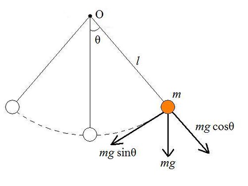
A simple pendulum can be defined as a mass m hanging from a
fixed point O by a taught massless string (or massless rod to ensure that
the system is indeed rigid) of length l. The following diagram
illustrates the situation.
From Newton's Second Law in angular form we have
where
and thus
Now, by the Parallel Axis Theorem we also have
Since l is our radius and mgsin(θ) is the force acting on
the pendulum perpendicular to l. The negative sign conforms to the
convention that torques in the clockwise direction are negative. Now we
have two ways to represent τ and they form the following equation which
can be simplified in the following way:
and we have the equation for the motion of our pendulum. Normally,
this is where one would assume that θ is small enough for the substitution
sinθ = θ. Our topic however is to assume that θ is not small and may
actually range from -π to π.
Now, since the motion of the pendulum is under a conservative force, we
can solve the motion problem by integrating and solving the energy
problem. First, we make the substitution
which is also customary in mechanics and is also algebraically
convenient. We then have
where c is the constant of integration.
In order to solve for c we will need to make some observations.
First, we can assume that at t0 the pendulum was pulled
up to some initial height h0, which will result in an
initial angular displacement of θ0. Thus, at t
0 we have angular speed equal to zero and θ equal to θ0. It may be of interest to point out here that since
there is assumed to be no friction on our pendulum, θ0
is also the maximum displacement of θ and the pendulum reaches
this displacement at the beginning/end of each period. This
observation
gives the following initial conditions to our differential equation
Which gives us
and thus our equation is
Likewise, one can derive the same conclusion by using the principle
of
conservation of energy
which saves them the pain of integration. Either way, solving
for dt we obtain
We now integrate from 0 to θ0 which will give us one
fourth of the period T.
We now make use of the trigonometric identity
which yields
Next we make the substitution
and solving for θ we obtain
we now make use of the fact that
which gives us
Now, by plugging this in to our original integral for T/4 we obtain
We make the substitution k = sin(θ0/2) which gives
us
which is a complete elliptic integral of the first kind.
We can now use a numerical approximator or a table to solve the
integral. I chose to use Mathcad for this. Complete elliptic
integrals of the first kind can be expressed as a special case
of the Gauss hypergeometric function multiplied by π/2 where
a = 1/2, b = 1/2, c = 1, and x = k where k is the same k we
used for our substitution in the previous equation. The Gauss hypergeometric function is typically denoted as
2F1(a,b;c;x)
where a, b, and c are real scalars such that if
a and b are nonzero then c must be nonzero as well and where
x is a real scalar such that -1 < x < 1. Now, we define K so that
K = (π/2)2F1(1/2,1/2;1;k^2)
and thus have our special case.
Now we have
by the preceding derivation and can now approximate our integral.
We now compare values for the period T of our pendulum between
the sinθ = θ approximation and our elliptic integral. Recall that
when we make the sinθ = θ approximation, we get an equation for the
period
where E stands for the estimated period. That is, E is an estimation
for T. The following calculations were done in Mathcad and then posted
on this website. In Mathcad, the command for the Gauss hypergeometric
function is fhyper(a,b,c,x) which is why that expression appears
below in place of 2F1(a,b;c;x).
The length l of the string is 4 ft in the example.
For π/6 we have
and our sinθ = θ approximation is pretty close the value given by
our elliptic function.
For π/2 we have
and we begin to notice that sinθ = θ approximation is not as good as
our elliptic function.
For 7π/8 we have
and the sinθ = θ approximation is way off.
Notice too that even for a value of θ as small as π/90 our
sinθ = θ approximation does not match exactly with the value given for
T by our elliptic function.
So, if you are going to approximate the period of a pendulum and you
do not wish to use a complete elliptic integral of the first kind,
you should make sure your pendulum has a small initial angle of
displacement; as small as possible in fact. However, if you do like
these integrals they can be very useful when applied to a simple
pendulum and come up in other applications of mechanics and
statistics.
References