Dustin Stevens-Baier
Comp 578
Assignment
#12
The K-means method is a prototype-based partitional clustering
technique that attempts to find a user-specified number of clusters K which are
represented by their centroids. The K-means method defines a prototype in terms
of a centroid which is usually the mean of a group of points and is typically
applied to objects in a continuous n-dimensional space. The basic
algorithm is as follows (gotten from the Text Book page 497).
1.
Select K points as initial centroids
2. repeat
3.
form K clusters by assigning each point to its closest
centroid.
4. Recompute the centroid of each
cluster.
5. until Centroids do not change.
An example
of the K-means algorithm using the iris data set and JMP 6 is as
follows:
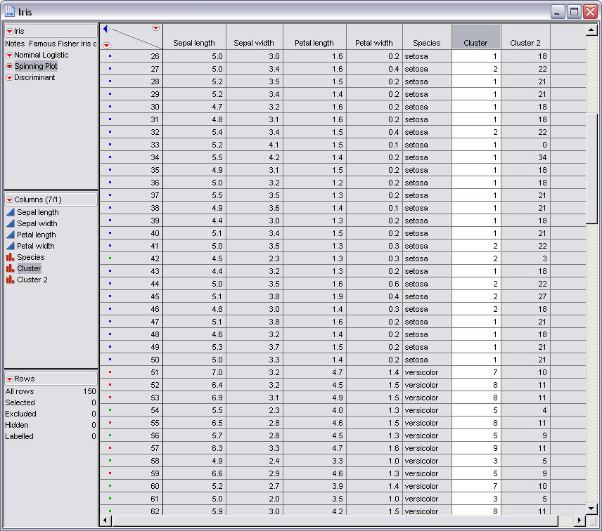
The above picture is a snapshot of the
iris data set. This data set is used to show the k-means in what is a
fairly easy to cluster example.
This image shows the four
variables sepal length, sepal width, petal length, and petal width that are used
in the clustering process.

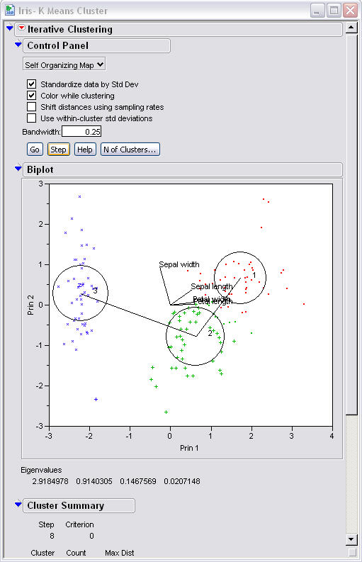
This is the first look at the k-means
before any steps are taken you can see two of the centroids that are clearly on
the blue and red areas. The third is very small and is labeled by the 2 in the
left hand corner on the green cluster.
After the next step you can see the
shapes begin to take place and start to move towards the middle of their
respective clusters. You can see that the green cluster is actually split
apart and that the centroid actually has none of the data points from he green
cluster in it.
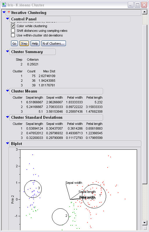
The next step
shows a slight shift of the centroids settling into their places.
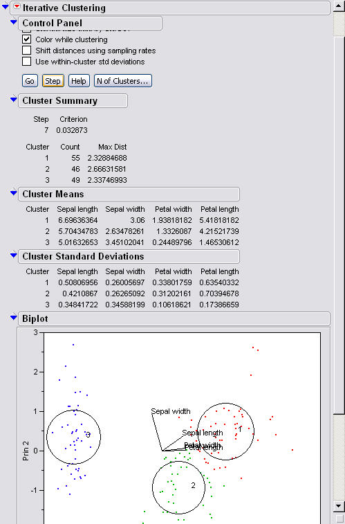
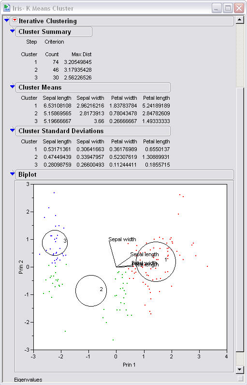
This is step seven which is the final step. Nothing changes after this step. You can see that it has
correctly labeled all of the data points in the clusters and that the centroids
are in the middle of their data points. One can see that not all of the
data does get encircled , outliers can also extremely
effect the clusters that are found. The
best solution is to eliminate the outliers before hand if possible. In
some situations this is not ideal because we may not know what the outliers are
or they might provide interesting info that we want to include in the
analysis.
In comparison the same data
set can be looked at in JMP from using self organizing maps. The data
looks as follows.
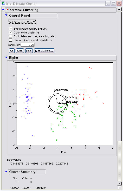
One can see that using Self Organizing
Maps has the three centroids placed in the middle of the data set.
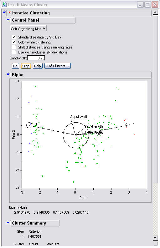
The next step in using SOMs shows that
there are now three centroids in the correct cluster areas.
The next step shows
that the circles are becoming more uniform in size and that they are closers
towards the centers of their clusters.
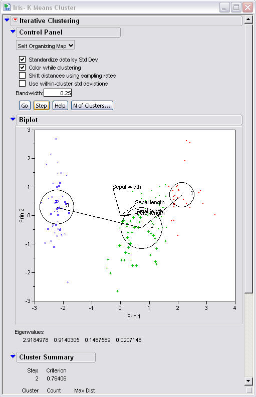
On step 7 the SOMs have finished moving
one can see that they have similar locations to the basic K-means but that they
have a few different data points inside the circles.
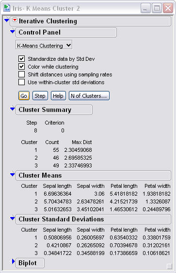
Looking at the data that comes from the basic K-means one
can see that cluster one has 55 points in it which is slightly off since we know
that there are supposed to be 50 points in each cluster. We can see that
this is a fairly accurate but not perfect. Cluster two is 46 data points
and cluster three is 49 data points. Another thing one can look at is the standard deviation of
the different variables for each cluster. You can see that cluster 3 is the tightest
of the three and there are a couple of values that are high,
cluster 1 sepal length and petal length, and cluster 2 petal length.
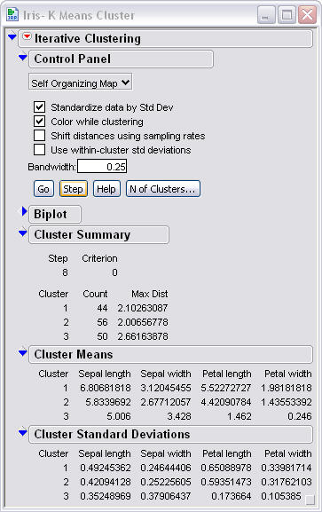
This is is cluster summary of the SOM
approach. It shows that the cluster were again a little off but pretty
close to the correct 50 data points per cluster. When comparing SOMs
standard deviations to the basic k-means algorithm. we can see that the
standard deviations are a little better, none are over the .7. It appears
that the SOM method gives slightly tighter clusters.
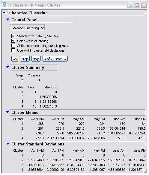
Another set of data that has much more error than the iris
set is the cholestrol data set. This set has four different treatments
however one of them gets left out and the data set becomes three clusters with
the fourth just being one point. It appears as if the data sets have
two many similar points so they overlap. One can also see that the standard deviations are
very high.
When computing
the
error of the K-means algorithm we could also use SSE, which is the sum of the
squared error. Given two different sets of clusters that are produced by
two different runs of K-means the most preferred one is the one with the
smallest squared error, because this means that the prototypes of this
clustering are a better representation of the points in their cluster.
Error can change when random centroids are used to start with.
Possible problems can
happen when initial centroids are chosen poorly. If they aren't picked correctly you
can get clustering that is not optimal. A very good example of this is in
the text on page 502. The basic problem is if the three clusters
have two of their centroids in the
same data area then the one of the sets will be divided when
it shouldn't be and another will be combined when it shouldn't. One way of dealing with
this problem is to run multiple runs with random initialization and choose the
one with the lowest SSE. This isn't very efficient but can give
us the best answer for a small number of K, with a relatively even
number of points in each cluster. If there is a larger number of K
then we probably will never get all of the clusters, also if one of the
clusters is significantly larger than the others it means that we will have
a harder time getting a selection not in the large
cluster.
One solution to this is to use a
hierarchal clustering technique. This technique has K clusters
extracted from the hierarchical clustering and the centroids of those clusters
are used as the initial centroids. This can work if the sample is small and K is
small as compared to the sample size.
Another problem with the
K-means algorithm is handling empty clusters. If no points are allocated
to a cluster during the assignment step then an empty cluster can be
obtained. If this happens then a replacement strategy needs to be
implemented. Two options for this are to replace the centroid from the
cluster with the highest SSE. This will usually reduce the SSE.