P (S = yes) = Sg[1 - P (S = no | B = bad, F = g)] * P (B = bad) * P (F = g) = .1 * 0.1 * .8 + 0 * 0.1 * 0.2 = 0.000016

The 1-nearest neighbor   y = + at x = 4.9 with D = 0.1 Class label +.

Majority vote 2-1 Class label -.

The 5-nearest neighbors are  y = + at x = 4.9 with D = 0.1,  y = - at x = 5.2 with D = 0.2,  y = - at x = 5.3 with D = 0.3 and y = + at x = 4.6 with D = 0.4.

Also you need to randomly select either y = + at x = 4.5 with D = 0.5 or y = + at x = 5.5 with D = 0.5 Since they are both pluses in this case it doesn't even matter.

Majority vote 3-2, it is class label +

The 9-nearest neighbors are y = + at x = 4.9 with D = 0.1, y = - at x = 5.2 with D = 0.2, y = - at x = 5.3 with D = 0.3, y = + at x = 4.6 with D = 0.4
y = + at x = 4.5 with D = 0.5, y = + at x = 5.5 with D = 0.5, y = - at x = 3.0 with D = 2.0 and  y = - at x = 7.0 with D = 2.0.

Also you need to randomly either y = - at x = 0.5 with D = 4.5 or y = - at x = 9.5 with D = 4.5 Since they are both minuses it doesn't really matter.

Majority vote 5-4, it is class label -

The 1-nearest neighbor is y = + at x = 4.9 with w = 100, Class label +.

The 3-nearest neighbors are y = + at x = 4.9 with w = 100, y = - at x = 5.2 with w = 25 and y = - at x = 5.3 with w = 11.11

Distance weigthed voting results in  100 - 25 - 11.11 = Class Label +

The 5-nearest neighbors are y = + at x = 4.9 with w = 100, y = - at x = 5.2 with w = 25, y = - at x = 5.3 with w = 11.11 and y = + at x = 4.6 with w = 6.25

Also need to select either y = + at x = 4.5 with w = 4 or y = + at x = 5.5 with w = 4

Distance weigthed voting results in   100 + 6.25 + 4 - 25 - 11.11 = Class label +

The 9-nearest neighbors are y = + at x = 4.9 with w = 100, y = - at x = 5.2 with w = 25, y = - at x = 5.3 with w = 11.11, y = + at x = 4.6 with w = 6.25,

y = + at x = 4.5 with w = 4, y = + at x = 5.5 with w = 4, y = - at x = 3.0 with w = 0.25, y = - at x = 7.0 with w = 0.25

Also need to randomly select either y = - at x = 0.5 with w = 0.05 or y = - at x = 9.5 with w = 0.05

Distance weigthed voting results in  100 + 6.25 + 4 + 4 - 25 - 11.11 - 0.25 - 0.25 - 0.05 = Class label +

16. (a) Demonstrate how the perceptron model can be used to represent the AND and OR functions between a pair of Boolean variables.

AND

X1	X2	y
0	0	-1
0	1	-1
1	0	-1
1	1	1

The AND function has on a graph four points one at (0,0), (0,1), (1,0), (1,1)  the first four a -1 and the last one is 1, A line can be drawn between the two batches of points. 

OR

X1	X2	y
0	0	-1
0	1	1
1	0	1
1	1	1

The OR function has on a graph four points one at (0,0), (0,1), (1,0), (1,1)  the first one is -1 and the last three are 1, A line can be drawn between the two batches of points. 



(b) Comment on the disadvantage of using linear functions as activation functions for multilayer neural networks.

Networks that produce linear output to their input can only classify and seperate problems that are linearly seperable. More complex activation functions allow these networks to model complex relationships between the input and output variables and can handle non-linearly seperable problems.

17.  You are asked to evaluate the performance of two classification models M1 and M2. The test set you have chosen contains 26 binary attributes labeled as A through Z.  table 5.14 shows the posterior probabilities obtained by applying the models to the test set.  As this is a two-class problem, P(-) = 1-P(+) and P(-|A,...,Z) = 1-P(+|A,...,Z).  Assume that we are mostly interested in detecting instances from the positive class.

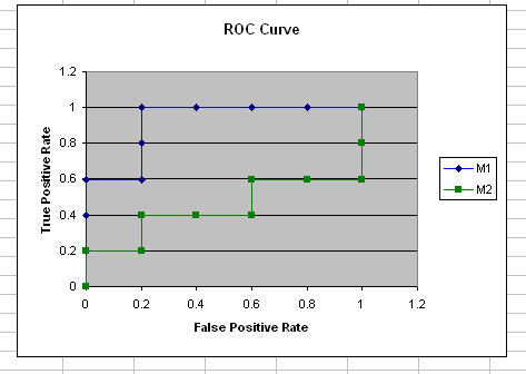
(a) Plot the ROC curve for both M1 and M2.  Which model do you think is better? Explain your reasons.

The M1 is better becuase it has far less Area Under the Curve  than M2. 

(b) For model M1, suppose you choose the cutoff threshold to be t=.5.  In other words, any test instances whose posterior probability is greater than t will be classsified as positive example.  Compute the precision, recall, and F-measure for the model at this threshold value. 

TP = 3, FN = 2, FP = 1, TN = 4

Precision = 3 / (3 + 1) = .75

Recall = 3 / (3 + 2) = .6

F1 = 2*3 / (2*3 + 1 + 2) = .67

(c)     Repeat the analysis for part c using the same cutoff threshold on model M2.  Compare the F-measure results for both models.  Which model is better?  Are the results consistent with what you expect from the ROC curve?

TP = 1, FN = 4, FP = 1, TN = 4

Precision = 1 / (1 + 1) = .5

Recall = 1 / (1 + 4) = .2

F1 = 2*1 / (2*1 + 1 + 4) = .29

M1 has the higher f measure therefor it is the better one.

(d) Repeat part (c) for model M1 using the threshold t = .1. Which threshold do you prefer, t = .5 or t = .1? Are the results consistent with what you expect from the ROC curve? 

TP = 5, FN = 0, FP = 4, TN = 1

Precision = 5 / (5 + 4) = .56

Recall = 5 / (5 + 0) = 1

F1 = 2*5 / (2*5 + 4 + 0) = .71

I like t = .5 better becuase it is just a little more towards the middle of all the threshold values.  For M1 t = .1 is at the beginning and t=.5 is in the middle.  For M2 t=.1 is in the middle and t=.5 is skewed towards the right just a little.