18. This exercise compares and contrasts soem
similarity and distance measures.
(a) For binary data, the L1 distance
corresponds to the Hamming distance; that is, the number bits that are different
between two binary vectors.� The Jaccard similarity is a measure of the
similarity between two binary vectors.� Compute the Hamming distance and
the Jaccard similarity between the following two binary vectors.
(b) which approach,
Jaccard or Hamming distance, is more similar to the Simple matching Coefficient,
and which approach is more similar to the cosine measure?� Explain.�
(Note: The Hamming measure is a distance while the other three masures are
similarities, but don't let this confuse you.)
Hamming
distance is more similar to the Simple Matching Coefficient.� Since the
Simple Matching Coefficient = 1- Hamming Distance.� This does not ignore
the 0-0 matches�unlike the Jaccard�similarity.
(c) suppose that you are comparing how similar two
organisms of different species are in terms of the number of genes share.�
Describe which measure, Hamming or Jaccard, you think would be more appropriate
for comparing the gentic makeup of two organisms.� Explain.� (Assume
that each animal is represented as a binary vector, where each attribute is 1 if
a particular gene is present in the organism and 0
otherwise.)
f11 matches should not occure becuase we
are dealing with seperate species.�� The other three should be there
alot.� Since the Jaccard ignores the f00
it isn't a good idea
to use it.� The Hamming code will take these into account.�
(d) If you wanted to compare the
gentic makeup of two organisms of the same species, e.g., two human beings, would
you use the Hamming, distance, the Jaccard coefficient, or a different measure
of similarity or distance? Explain. (Note that two human being�share >
99.9% of the same genes.)
Because we are
comparing the same species the dominant factor will be f11.� I
would not use the Hamming method becuase it doesn't seem to give a good
representation, it would take the f00
into account and we don't want that.� It seems
like the best one would actually be correlation since it gives a decent
distribution that can get close to 1.
19. For the following
vectors, x and y, calculate the indicated similarity or distance
measures.
1. Obtain one of the data sets available at the UCI
Machine Learning repository and apply as many of the different visualiation
techniques described in the chapter as possible.� The bibiliographic notes
and book Web site provide pointers to visualization software.
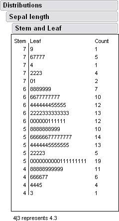
It seemed to make a lot of since to use the classic iris
set.� I also used Jump 6.0 free trial download since I already have this
program for Pattern recognition.� A good reason to use jump is that the
sample data is already created and we just need to do some analyzing and
graphing.
�
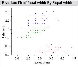
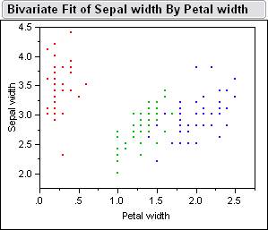
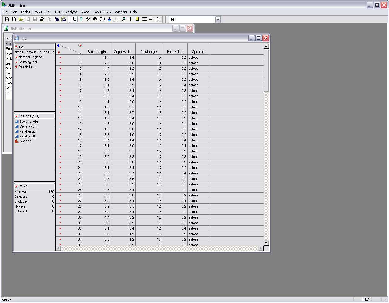
Here
is a picture of the sample data inside jump.� Below is the Bivariate Fits
of all the different combinations petal length, petal width, sepal width, sepal
length.
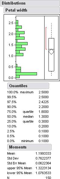
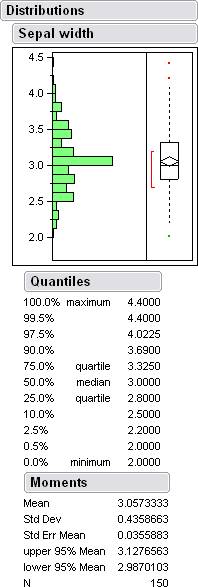
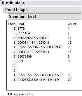
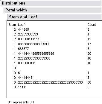
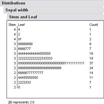
Here are some histograms along with some data from jump.
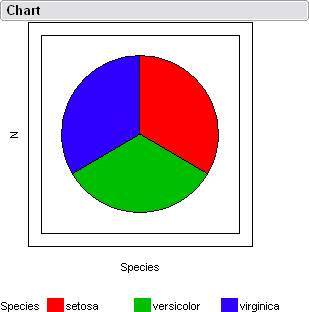
A pie chart which isn't all that useful in this case since the sample has the same
amount of data for each type of flower.
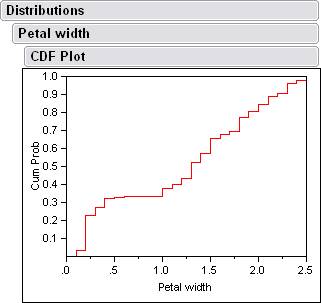
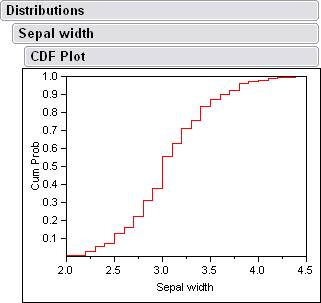
There are also cdf plots that come from the histograms.
 �
�