
Dustin Stevens-Baier
Comp 569
Assignment #4
A.1. Wikipedia search: Bayesian Network
A bayesian network is a probabilistic graphical model that represents a set of variables and their probabilistic independencies. (This is from wikipedia, although most stats books have some variation of the above sentence.) Bayesian networks are directed acyclic graphs whose nodes represent variables and the arcs are the conditional independencies.
Explain Example: Sprinkler
When discussing the sprinkler example illustrated on wikipedia we first must outline the problem. The grass can be wet if one of the following two conditions are met, it's raining or the sprinkler is on. Also when it is raining the sprinkler is usually not on.
In this image from wikipedia one can see the graphical representation next to the truth table. You can see that the rain has an effect on the grass being wet and the sprinkler being on. but not the other way around. There are some truth tables that show us the probability of the grass being wet given the conditions being either true or false.
We can use the model to answer the question What is the likelihood that the sprinkler is on given the grass is wet? ( A slight derivation from the example problem)
P(S=T|G=T) = P(G=T, S=T)/P(G=T) = P(G=T,R,S=T)/P(G=T,R,S) = ((.99*.01*.2=.00198) + (.9*.4*.2=.072)) / (.00198+.288+.072+ 0) = .07398/ .36198 =20.44%
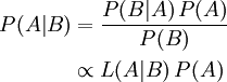
A.2. Wikipedia search: Bayes' Theorem
Bayes' Theorem is a result in probability theory, which relates the conditional and marginal probability distributions of random variables (again from wikipedia although a stats book would be just as good). The probability of an event A conditional on another event B is generally different from the probability of B conditional on A. However, there is a relationship between them. Bayes' theorem is the statement of that relationship:
Explain Examples: Cookies
First, lets again list the example. Suppose there are two bowls full of cookies. Bowl #1 has 10 chocolate chip cookies and 30 plain cookies, while bowl #2 has 20 of each. Fred picks a bowl at random, and then picks a cookie at random. We may assume there is no reason to believe Fred treats one bowl differently from another, likewise for the cookies. The cookie turns out to be a plain one. How probable is it that Fred picked it out of bowl #1?
To better illustrate Bayes' theorem lets rephrase the question in the correct form. What's the probability that Fred picked a cookie from bowl one given that he picked a plain cookie. So we are looking to compute Pr(A|B).
Pr(A) is .5 since Fred is treating both bowls equally.
Pr(B) = .75 * .5 + .5*.5 = .625 we get this by multiplying the probability of getting a plain cookie in that bowl by the probability of choosing that bowl.
Pr(B|A) = .75 the probability of getting a plain cookie if we choose bowl 1.
Pr(A|B) = .75 * .5 /.625 = .6 using Baye's Theorem.
We can also do the cookie problem with different percentages. Lets say the first bowl actually has 5 chocolate chip cookies and 35 plain ones. While the second bowl has 30 chocolate chip cookies and 10 plain ones.
Pr(A) = .5 still because we have two bowls.
Pr(B) = .875*.5 + .5*.25 = .5625
Pr(B|A) = .875
Pr(A|B) = .875*.5/.5625 = .78 So you can see that this result makes some sense if we increase the number of plain cookies in bowl one and decrease the number of plain cookies in bowl two the percentage should go up.
Drug Testing
Bayes' theorem is useful in evaluating the result of drug tests. Suppose a certain drug test is 99% accurate, that is, the test will correctly identify a drug user as testing positive 99% of the time, and will correctly identify a non-user as testing negative 99% of the time. This would seem to be a relatively accurate test, but Bayes' theorem will reveal a potential flaw. Let's assume a corporation decides to test its employees for opium use, and 0.5% of the employees use the drug. We want to know the probability that, given a positive drug test, an employee is actually a drug user. Let "D" be the event of being a drug user and "N" indicate being a non-user. Let "+" be the event of a positive drug test.
Pr(D) The probability of being a drug user as stated is .005
Pr(N) the probability of being a non-user as stated is .995 (1-.005)
Pr(+|D) the probability that the test is positive given theft the employee is a drug user as stated .99
Pr(+|N) the probability that the test is positive for a non user is .01 as stated (1-.99)
Pr(+) the probability of a positive test .01 * .995 = . 00995(N) and .99*.005 = .00495(D) Then add these together and we get .0149 or 1.49%
Using Baye's Theorem
P(D|+) = .99*.005 /(.99*.005+.01*.995) = .3322 The bottom figure is the P(+) we just calculated
This illustrates how high the false positives can be when a test is testing something so rare.
Monty Hall
We are presented with three doors - red, green, and blue - one of which has a prize. We choose the red door, which is not opened until the presenter performs an action. The presenter who knows what door the prize is behind, and who must open a door, but is not permitted to open the door we have picked or the door with the prize, opens the green door and reveals that there is no prize behind it and subsequently asks if we wish to change our mind about our initial selection of red. What is the probability that the prize is behind the blue and red doors?
This problem is essentially you have three doors and a prize behind one of the doors. You get to choose a door first, so you have a 1/3 probability of being write and each of the other doors has a 1/3 probability of being write.
Ar = Ab = Ag = 1/3.
Then the host shows you one of the two doors that you didn't choose and it has no prize. Then asks you if you want to change. Because nothing has changed about the door we choose Ar it is still 1/3. but since the other two doors which had a probability of 1/3 + 1/3 of being right has one of the doors removed from the equation Ag.The probability is know 2/3 for Ab.
This problem can be demonstrated in a variety of ways with different data. A good example is to make the problem be four doors. Thus making each one have a 25% probability of having the prize. So once you select one there is a 75% chance the prize is behind a door that you didn't choose. Then when one door is opened that you didn't choose, the probability is still 75% but the number of doors is now 2 instead of 3. Thus making each door 37.5% likely, while the door you originally picked is still 25%.
Part II - DEPENDING ON WHERE YOU REVIEW THE NOTES THIS DATA CHANGES
(In the notes package purchased in the school store the data varies from the notes from the links page)
The nodes are four different categories in this problem. First are all the input nodes these are the primary evidential variables: DECOR, TABLE SETTING, SURFACE CLEANLINESS, AIR, SOUNDS, CLIENTELE, MENU, PRICES, SERVICE. they are used to compute the next set of nodes. The next set of nodes is computed using a combination of the primary evidential variables, and is called the lumped evidential variables, these are: POPULARITY, ELEGANCE, ARTISTRY, CLEANLINESS. The Lumped Evidential Variables are used to predict the next set of nodes, these are called Predicted Component Variables and they are: TASTE, TEXTURE, APPEARANCE, QUANTITY, CORRECTNESS, NUTRITION, HYGIENE. Finally all of these combine for the output node also called Predicted Summary Variable: OVERALL FOOD QUALITY.
INPUT NODES
DECOR- .5 prior probability and .9 current probability
This is to be rated high when the decor is pleasing and tasteful. This is, of course, a subjective measure that depends on the .
TABLE SETTING- .5 prior and .8 current
This is rated high when the tables are in a nice, neat, arrangement and are set with a respectable silverware, glasses, flowers, napkins, table cloth, etc.
SURFACE CLEANLINESS- .8 prior and .8 current
This is high when things appear clean. This is not to be confused with hygiene since we cannot see the cook and we cannot see if hands are washed etc.
AIR - .6 prior and .6 current
This is high when the air looks clear and smells fresh. It may be difficult to smell the air from the outside, so this may depend only on visual measurement
SOUNDS- .5 prior and .5 current
This is high when there is very little noise and higher yet if there is a pleasing music. Again, this is a very subjective measurement.
CLIENTELE .5 prior and .9 current
This is high when the people that are a1ready in the restaurant are apparently well dressed, peaceful and friendly looking. There may be other knowledge of the clientele, such as references from friends etc, that may play and indirect role here.
MENU- .5 prior and .5 current
This is high when the menu appears impressive (nice print, not tattered, etc) and there is a sufficient selection of meals without offering too many. It may seem clear to some that a menu that includes too much variety, suggests inferior ingredients, but this is a very subjective measurement.
PRICES- .5 prior and .9 current
This is high when the prices seem reasonable, based on your knowledge of prevailing prices for that region of the city, or country.
SERVICE- .3 prior and .9 current
This is high when the staff appears numerous and friendly and well dressed and clean.
LUMPED EVIDENTIAL VARIABLES
POPULARITY- .5 prior and .6 current, two sub expressions ARC SOUNDS 3.0 1.0 and ARC CLIENTELE 1.0 .24 these are to be combined using the independent influences (INDEP). The 3.0 next to sounds is the sufficiency factor so if the current probability was 1.0 it would be multiplied by 3.0. The second number 1.0 is the necessity factor. So ARC CLIENTELE has a sufficiency factor 1.0 and a necessity factor of .24.
ELEGANCE- .5 prior and 0.0 current, ARC DECOR 3.0 sufficiency and .5 necessity, ARC TABLE SETTING 1.0 sufficiency and .74 necessity, ARC SOUNDS 1.5 sufficiency and .74 necessity, ARC CLIENTELE 1.0 sufficiency and .5 necessity, ARC MENU 1.24 sufficiency and .74 necessity, ARC PRICES 1.24 sufficiency and .74 necessity, and ARC SERVICE 1.0 sufficiency and .5 necessity.
ARTISTRY- .5 prior and .9 current, ARC DECOR 1.0 sufficiency and .5 necessity, ARC TABLE SETTING 1.0 sufficiency and .5 necessity, ARC MENU 1.5 sufficiency and .74 necessity, ARC SERVICE 1.0 sufficiency and .5 necessity.
CLEANLINESS- .7 prior and .7 current, ARC SURFACE CLEANLINESS 1.5 sufficiency and .2 necessity, ARC AIR 1.5 sufficiency and .5 necessity.
PREDICTED COMPONENT VARIABLES
TASTE- .6 prior and .6 current, ARC POPULARITY 3.0 sufficiency and .7 necessity, ARC ELEGANCE 1.5 sufficiency and .8 necessity.
TEXTURE- .6 prior and .6 current, ARC POPULARITY 3.0 sufficiency and .7 necessity, ARC ELEGANCE 1.0 sufficiency and .5 necessity.
APPEARANCE- .5 prior and .5 current, ARC ARTISTRY 3.0 sufficiency and .4 necessity
QUANTITY- .5 prior and .5 current, ARC POPULARITY 1.5 sufficiency and .5 necessity
CORRECTNESS- .5 prior and .5 current, ARC ELEGANCE 1.0 sufficiency and .7 necessity
NUTRITION- .6 prior and .6 current, ARC POPULARITY 1.1 sufficiency and .7 necessity, ARC ELEGANCE 1.8 sufficiency and .8 necessity.
HYGIENE- .8 prior and .8 current, ARC CLEANLINESS 1.0 sufficiency and .1 necessity
PREDICTED SUMMARY VARIABLE
OVERALL FOOD QUALITY- .5 prior and .5 current, ARC TASTE 3.0 sufficiency and .3 necessity, ARC TEXTURE 1.0 sufficiency and .5 necessity, ARC APPEARANCE 1.0 sufficiency and .3 necessity, ARC CORRECTNESS 1.3 sufficiency and .8 necessity, ARC QUANTITY 1.2 sufficiency and .8 necessity, ARC NUTRITION 1.0 sufficiency and .3 necessity, ARC HYGIENE 1.5 sufficiency and .2 necessity
Another example would be to determine the skill of a baseball player lets say a positional player to make things more comparable. The Output node would be OVERALL PLAYER QUALITY and the input nodes would be COST, UNIFORM, BATTING AVERAGE, HOMERUNS, RBI, WALKS, STOLEN BASES, and FIELDING. The predictor nodes would be STRENGTH, SPEED, EYESIGHT, FLEXIBILITY, HEIGHT, WEIGHT, and APPEARANCE. Then the lumped nodes would be MEDICAL, POPULARITY, ATHLETICISM, GRACEFULLNESS, and PRESENTABILITY. Medical predicts eyesight. Popularity would help predict everything but in varying amounts. Athleticism would help predict everything but eyesight and flexibility. Gracefulness predicts, speed, flexibility, weight and height. Presentably predicts height, weight, and appearance. Cost is factored into popularity and presentably. Uniform is factored into height, weight, and appearance. Batting Average is factored into popularity, athleticism and gracefulness. Home runs are factored into popularity and athleticism. RBI is factored into popularity and athleticism. Walks are factored into Medical. Stolen bases are factored into Athleticism and Gracefulness. Fielding is factored in Athleticism, Medical, Gracefulness.
Obviously there are many other interpretations of these rules but this is an outline that I think can be followed relatively easy.
Resources:
http://hawk.cs.csuci.edu/william.wolfe/ucd/engineering/cse/graduate/courses/comp581/summer07/assignments/TravelersRestaurantSelection_Notes.pdf
http://hawk.cs.csuci.edu/william.wolfe/ucd/engineering/cse/graduate/courses/comp581/summer07/assignments/TravelersRestaurantSelection_Tanimoto.pdf