How does it work ?
» In many cases, we can't have the distribution of an estimator.
Bootstrap method allows to approximate this distribution, making a numeric simulation, when the number of observations is relatively low.
» Here we build a sample according to the distribution choosen.
The size of this initial sample is n=100.
All the distribution are generated from U( [0;1] ) and using Box-Muller method for gaussian distribution.
» Then we start with the bootstrap method. We create N=1000 samples based on the initial sample by picking an element and replacing it. The size of the N samples is m=50 (m< n).
» Here we want to estimate the variance.
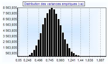
» The first natural choice is the empirical variance. The program calculates all the empirical variances of the N samples. Then we can see the distribution on the top histogram. This shows the distribution of the empirical variance's estimator.
» We build now a new estimator, called 'plugging estimator' , obtained by replacing, in the theorical variance, the parameters by estimators (in this program i use the empirical mean).
We can see the distribution of the plugging estimator in the low histogram. 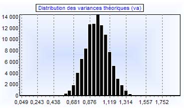
» As we can see on the histograms, the distribution is really more tightened with the plugging estimator, and the variance of the plugging estimator is always inferior than the variance of the empirical estimator (empirical variance).
» You can also click on the button "affiner la distribution". Consequently, every 0.01 seconds, it creates a new initial sample, 1000 new bootstrap samples, and calculates the empirical and theorical (plugging) variances. Then the new histogram is pilled up on the old one and we can see an application of the Central Limit Theorem. The estimations are more precise and tend to their true values (CLT).
SAMPLING ALGORITHMS
» In all the cases, U is a random number between 0 and 1 (generated by uniform[0;1] ).
Bernouilli Distribution
for i:=1 to 100 do
begin
u:=random
if u<teta then v[i]:=1;
end;
|
|
Binomial distribution:
for i :=1 to 100 do
begin
for j:=1 to 100 do
begin
u:=random
if u<teta then v[i]:=v[i]+1 else v[i]:=v[i];
end;
end;
|
Poisson distribution:
for i:=1 to 100 do
begin
n:=1;
u:=random;
while u > exp(-param_lambda) do
begin
u:=u*random[0;1];
inc(n)
end;
v[i]:=n-1;
end;
|
|
Gaussian Distribution:
for i:=1 to 100 do
begin
w:=random;
u:=random;
v[i]:=(s*(sqrt((-2)*Ln(u/1000))*cos(2*Pi*(w/1000)))) + m;
end;
|
Expontial Distribution:
for i:=1 to 100 do
begin
u:=random;
v[i]:=(ln(u)*(-(1/lambda_exp)));
end;
|
|
Geometric Distribution:
for i:=1 to 100 do
begin
u:=random;
v[i]:=ln(u)/ln(teta_geo);
end;
|
Pareto
for i:=1 to 100 do
begin
u:=random;
v[i]:=alpha_pareto/(Power(beta_pareto,u));
end;
|
|
COMMENTS AND PROBLEMS
As you can see, there are some problems with Geometric and Pareto Distibution... The empirical variance is better than the plugging variance, wich is .... a mistake.
If you want you can see the sources and so you can correct it and send me back the code.
For the plugging variance, all the estimators aren't unbiaised.
In fact, for exemple with the Berouilli's distribution, we can observe that
the variance of plugging wariance is better with an biaised estimator than with the unbiaised estimator (wich is the same than the empirical variance by the way).
So I kept the biaised estimators for all the estimators.
You can see the estimators in the source code.
___________________________ » Main lines of the program: - sampling function (according to the distribution choosen).
- bootstraping function.
- Calcul of the plugging variance function (according to the distribution choosen).
- maximum and effectif functions (to create histograms).
- You can change the parameter's values in the distribution choosen. ___________________________ » Nota:
In this beta program, there are some mistakes.
If you want to improve it, you can download the sources and send me back the corrections.
Thanks David.
|