Loop quantum cosmological models have been developed in the last decade by especially by Martin Bojowald and Abhay Ashtekar. Even the most simple models of loop quantum cosmology are still not fully understood, but the field has captured a lot of interest and a lot of research is ongoing now, providing many new results.

Loop quantum gravity

Loop quantum cosmology is based in loop quantum gravity. This is a theory of quantum gravitation that canonically quantizes general relativity, in a different manner, however, than canonical quantum gravity. The main difference is the choice of different variables to describe the gravitational degrees of freedom that lead also to different consistency conditions for the application of Dirac's quantization procedure in the theory.

The new variables are called Ashtekar variables. Instead of the spatial metric one uses the densitized triad (an orthonormal spatial frame) and its canonical conjugate Ashtekar connection, defined with the spin connection and extrinsic curvature. It has to be noted that unless to the spatial metric, a triad, being a frame, knows about the orientation of space. The orientation will be important in the dynamics of the universe near the singularity. The variables that are used to set up the Dirac quantization procedure are however other ones that are build defining holonomies of the connection and fluxes of the triad. The important thing to know is that the basic phenomenological feature of the theory is that quantum observables of volume and area have a discrete spectrum.

Loop quantum cosmology and the different regimes

Loop quantum cosmology is also basically different than canonical quantum cosmology. In canonical quantum cosmology the Dirac quantization procedure is applied after symmetry reduction to minisuperspace. This means that the classical space of solutions is reduced first to the Friedmann-Robertson-Walker solutions that fulfil the cosmological principle. Afterwards, the quantization procedure is performed taking as the dynamical variables the scale factor and its conjugate momentum. This leads to the definition of quantum observables that act on the wavefunction of the universe. The hamiltonian constraint is equivalent to the first Friedmann equation in minisuperspace and is imposed as a quantum condition on the wavefunction of the universe.

In loop quantum cosmology, however, the symmetry reduction is performed after the quantization procedure and not before. It is searched for homogeneous and isotropic representations of the quantum algebra of observables. The hamiltonian constraint is derived from the full theory. In order to extract physical content of the equations it is made use of a semiclassical approximation, that in the limit of great scale factor gives rise to the classical Friedmann-Robserton-Walker solutions. The hamiltonian constraint is thus equivalent to the first Friedmann equation only in the appropriate regime.

The fact that the operators in loop quantum cosmology are rooted in the full theory provides the discrete framework necessary to eliminate singularities that appear in the classical equations and that were not eliminated in canonical quantum gravity. This is the essential phenomenological difference with respect to canonical quantum cosmology. The hamiltonian constraint in loop quantum cosmology is usually expressed in two different forms: (i) on the one hand it is possible to express it based on the dicrete isotropic and homogeneous volume operator, without making any approximation, giving rise to a difference equation and (ii) on the other hand it is possible to express it in a semiclassical approximation with so called effective equations, giving rise to equations modified classical equations.

Thus, loop quantum cosmology describes the dynamics of the universe in three different regimes:

• A discrete regime. This is applicable near the classical singularity. The universe evolves in a discrete time, from one time instant to another. Its evolution is described by difference equations. Thus the classical singularity is resolved with a deterministic evolution.
• A semiclassical regime. This is applicable near the Planck time. The evolution of the universe is described by differential equations that are similar to the classical equations, but with some modified terms. However, the differences with respect to classical cosmology are remarkable as we will see.
• A classical regime. This is applicable for a time greater than the Planck time. This corresponds to the classical cosmological evolution.

The discrete regime

In the discrete regime of loop quantum cosmology the dynamics of the universe is described by a difference equation. This equation corresponds to the Hamiltonian constraint H(i) F(i) = 0, with H the Hamiltonian and F the wavefunction of the universe that is written as a linear combination of volume eigenstates labeled by some integer i.

Note that the state of the universe can be in a linear combination of the volume eigenstates, but in its time evolution the universe is expected to evolve from one volume eigenstate into another. Thus, time evolution in loop quantum cosmology requires the identification of an internal time variable which is usually taken to be a comoving volume in analogy to the classical evolution of the universe.

In general, a state F(i = io) depends on initial conditions that are given by the previous states io - 4 and io - 8, and the space of solutions extends beyond the singularity for i < 0. The singularity is solved with the discrete time evolution. At intuitive level, the universe starts in a collapsing branch and evolves through a discrete phase bouncing to the expanding branch.

The quantum evolution through the singularity is strongly model dependent, but it uniquely yields the wavefunction on the expanding branch if initial values on the contracting branch are posed. However, for io = 0 all H(i) vanish, leaving no initial condition at the singularity. Thus, loop quantum cosmology implements dynamical initial conditions that have not to be introduced at the singularity as an additional assumption in the model.

Moreover, the space for wavefunctions F(i) knowns about the orientation of space-time and at the transition between the two branches, the orientation of space changes. What exactly happens during the transition depends on the concrete matter model and results are currently unclear (e.g. a parity violating matter Hamiltonian may imply a change in the behaviour of matter due to the change of orientation of space-time).

The semiclassical regime

In the semiclassical regime the discrete operators can be approximated by continuous functions to recover usual differential equations and make it possible a more easy handling of the mathematical framework. At least for simple models such as homogeneous and isotropic minisuperspace with scalar field the resulting equations of motion differ from the classical ones in a semiclassical regime, but they are equal to the classical equations for great values of the scale factor.

To illustrate how this difference between classical and semiclassical equations looks like lets take a look to the Klein-Gordon equation. Note however that the semiclassica modifications also affect the FRW equations. The classical Klein-Gordon equation for a scalar field f with self-interacting potential V(f) reads (H = a ' / a, the Hubble parameter):

f ' ' - 3 H f ' + dV(f)/df = 0

Near the point of equilibrium this equation describes the behaviour of a damped harmonic oscilator with a friction that depends on the expansion of space-time (the Hubble parameter). The semiclassical equation reads:

f ' ' - ( d[log D(a)]/da ) a ' f ' + a3 D(a) dV(f)/df = 0

The function D(a) is a very complex one and depends on some ambiguities. For large scale factor D(a) ~ 1/a3 and the equation is the same as the classical above.

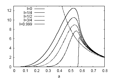
The function D(a) (from gr-qc/0601085)

Near the point of equilibrium and for small values of the scale factor the modified Klein-Gordon equation shows the behaviour of a harmonic oscilator that is driven by antifriction generating a repulsive effect. This drives the field to greater values of the potential providing the appropriate condition for inflation (high potential energy), until the semiclassical phase ends and the behaviour becomes the classical one (friction):

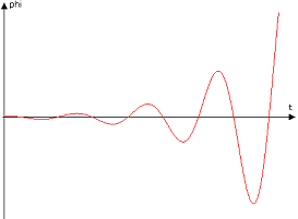
Antifriction

Thus, in the semiclassical regime the parameter of state of the scalar field is driven to values w = -1 and even w < -1 (those values that arise in case of high potential energy). But it can be shown that the modified equations lead to a modified equation of state of matter that implies w < -1 and w = -1 for small values of the scale factor for any kind of matter (and not only for scalar fields with self-interacting potentials). This is a very interesting result. Loop quantum cosmology provides therefore a framework in which inflation may take place naturally and without the need of a scalar field.

Some further reading

• M. Bojowald, Loop Quantum Cosmology, gr-qc/0601085
• M. Bojowald, Universe scenarios from loop quantum cosmology, astro-ph/0511557
• M. Bojowald, Isotropic Loop Quantum Cosmology, qr-qc/0202077
• D. G. Green, W. G. Unruh, Difficulties with Re-collapsing Models in Closed Isotropic Loop Quantum Cosmology, gr-qc/0408074
• P. Singh, Effective State Metamorphosis in Semi-Classical Loop Quantum Cosmology, gr-qc/0502086
• G. M. Hossain, On Energy Conditions and Stability in Effective Loop Quantum Cosmology, gr-qc/0503065