Updated: January 28, 2008

Electrostatic Response of an Arbitrary Dielectric Object


A numerical method is introduced for determining the dipole moment induced when an arbitrary object with specified position dependent permittivity is placed in an asymptotically uniform static electric field. This allows the polarizability of a nonspherical inhomogeneous nanoparticle (needed for light scattering cross sections) to be estimated in the static field approximation.


1. Introduction:
   Nanoparticles are very small compared to the wavelength of the laser light used to excite them in Raman and Brillouin light scattering experiments. For this reason, at an instant of time the electric field in a given region enclosing a nanoparticle may be regarded as a uniform static electric field. The nanoparticle has a dielectric constant which differs from that of the surrounding glass matrix. For this reason there will be a spatial variation of the electric field in the interior and vicinity of the nanoparticle. This electric field induces polarization and consequently bound charge on the nanoparticle which has a dipole moment. It is this electric dipole that oscillates so as to radiate emitting Rayleigh scattered light (with the same wavelength as the incident light). Acoustic vibrations of the nanoparticle lead to variations in the dielectric response of the nanoparticle on a timescale that is very long relative to optical timescales. As the nanoparticle slowly vibrates, its dielectric response will change so that the strength or phase of the induced dipole moment will also change. This leads to Raman or Brillouin scattered light whose frequency is slightly above or below that of the incident laser.
   The true electrodynamic character of the process is ignored in what follows in order to make the calculations tractable. However this approximation is justifiable for several reasons:

(1) The smallness of the nanoparticle relative to the laser wavelength
(2) The slowness of the nanoparticle vibration relative to optical time scales.
(3) The large separation of neighbouring nanoparticles with respect to their diameter.
(4) Even though magnetic fields are associated the incident electromagnetic wave, they are not relevant to the induced dipole moment and consequent Rayleigh and Raman (or Brillouin) scattering.

   Consider a single instant of time. Consider also a region surrounding the nanoparticle over which the incident electric field is approximately constant. The incident electric field Einc has components Eincx, Eincy and Eincz. If only glass (and no nanoparticle) were present in the region then the electric field would be constant within the region (ignoring electrodynamic effects). The effect of the variation of the dielectric response of the nanoparticle material relative to that of the glass is that the electric field varies in and close to the nanoparticle.
   In the following sections, a numerical method is introduced for determining the resulting electric fields associated with the nanoparticle as well as the dipole moment of the nanoparticle. In addition, exact results for special cases are recalled and compared with results of the numerical method.

2. Spherical Harmonic Transform:
   Consider a nanoparticle that is "roughly" spherical in shape and "roughly" centered at the origin of the coordinate system. Even though the nanoparticle is not a sphere, and may not even have a clearly defined surface, a general estimate of its radius is given by Rp. The electric field is E(r). Because of the static approximation E = -∇ V where V(r) is the electric potential.
   The motivation for introducing the word "roughly" twice above is to justify the use of a spherical harmonic expansion for the potential V which is dominated by components with slow angular variation. However, notwithstanding this any potential could with generality be expressed in the form:

V(r,θ,φ) = Σ
lm
 alm(r) Slm(θ,φ)
[2.1]
where Slm(θ,φ) are "real spherical harmonics" (also known as "tesseral harmonics") which are real-valued functions here defined as:
  Slm = -0.707107 (Ylm + Ylm* ) = -sqrt(2) Re(Ylm) [ m > 0 ][2.2]
  Slm = Ylm [ m = 0 ][2.3]
  Slm = 0.707107 i (Ylm - Ylm* ) = -sqrt(2) Im(Ylm) [ m < 0 ][2.4]
where i = sqrt(-1), * denotes the complex conjugate and Ylm(θ,φ) are the conventionally defined complex valued spherical harmonic functions: [ Reference: mathworld.wolfram.com We use the sign convention for the spherical harmonics as in Abramowitz and Stegun, Gradshtyn and Rhyzhik and J. D. Jackson. However, the definition of the Slm is not standard and has been selected for convenience in our present purposes.]

Ylm(θ,φ) = sqrt( [(2l+1)/(4π)] [(l-m)!/(l+m)!] ) Plm(cos(θ)) ei m φ
[2.5]
   Note that m can vary from -l to l in this expression. Zero factorial is 1. The Condon-Shortley phase factor of (-1)m is built into our definition of Plm the associated Legendre functions.
   There are orthonormality conditions for both Ylm and Slm:
∫∫ Ylm (YLM)* sin(θ) dθ dφ = δlL δmM
[2.6]

∫∫ Slm SLM sin(θ) dθ dφ = δlL δmM
[2.7]
where δij is the Kronecker delta and the asterisk (*) denotes the complex conjugate.

Table I: Real Spherical Harmonics
S0 0 = 0.282095
S1 0 = 0.488603 cos(θ)
S1 1 = 0.488603 sin(θ) cos(φ)
S1-1 = 0.488603 sin(θ) sin(φ)
S2 0 = 0.630783 (1/2) (3 cos(θ)2 - 1)

   In macroscopic electrostatics the permittivity ε and the fields E, D and the polarization P are related through
D = ε E
[2.8]
and
P = εor-1) E
[2.9]
where εo = 8.854187817×10⁻¹² is the permittivity of free space and ε = εr εo, where εr is the "relative permittivity."
   The above relations are assumed here. However at microscopic scales these relations break down. One mechanism for this is Thomas-Fermi screening, the result of which the macroscopic theory doesn't work over very short distances. The motivation for employing this assumption is that nanoparticle sizes are large enough that a macroscopic treatment of the electrodynamics is plausibly justifiable.
   The permittivity is a function of position. This spatial variation has two reasons:
(1) the permittivity of the nanoparticle is different from the permittivity of the surrounding glass matrix.
(2) vibrations of the nanoparticle will lead to elastic strains which will cause small time dependent variations of the permittivity. (These periodic variations have a timescale on the order of 3 ps, which is 1000 times longer than the period of the incident laser light beam)
   Once again, motivated by the roughly spherical shape of the nanoparticle about the origin, a real spherical harmonic expansion is employed:
ε(r,θ,φ) = εo Σ qlm(r) Slm(θ,φ)
[2.10]
It also turns out to be convenient to introduce the logarithm (base e) of the permittivity b = log(ε/εo). This has the expansion:
log(εr(r,θ,φ)) = b(r,θ,φ) = Σ clm(r) Slm(θ,φ)
[2.11]
Note that the coefficients clm(r) and qlm(r) are dimensionless, while the alm(r) are in volts.
   While V(r) may have non-analytic variation in the vicinity of the surface of the nanoparticle due to rapid spatial changes in ε(r), we suppose that V(r) is smooth at the origin with the following series expansion:
lim
r→0
V(r,θ,φ) = Σ dlm r l Slm(θ,φ)
[2.12]
   Finally, we suppose that sufficiently far away from the nanoparticle the permittivity again becomes constant. In this region the electric field is supposed to reach a spatially constant value, but formally the potential can be expanded in the large r limit as:
 lim
r→∞
V(r,θ,φ) = Σ elm r l Slm(θ,φ)
[2.13]
The x, y and z incident (far away) electric field components are related to e1,0, e1,1 and e1,-1 as follows:

  Eincz = -0.488603 e1 0[2.14]
  Eincx = -0.488603 e1 1[2.15]
  Eincy = -0.488603 e1 -1[2.16]

3. Integration of Coulomb's Equation:
   The basis of the calculation is that there are no free charges associated with the nanoparticle, although there will be some bound charge as a result of the induced polarization. Thus ρf = 0, in which case ∇·D = 0 but D = εE, so ∇·(ε E) = 0. Note further that E = -∇V, so that
∇ · (ε (∇ V)) = 0
[3.1]
A product theorem of vector differentiation says that:
∇ · (ε E) = ε (∇·E ) + E · (∇ε)
[3.2]
with the final resulting differential equation:
ε ∇2V + (∇V)·(∇ε) = 0
[3.3]
Next, divide through by the function ε(r).
2V + (∇V)·((∇ε)/ε) = 0
[3.4]
But if b = log(ε/εo) = log(εr) then ∇ b = (∇ε)/ε
In this case
2V + (∇V)·(∇b) = 0
[3.5]
   Supposing b(r) = log(ε(r)/εo) to be known, it will be this partial differential equation which will be solved to yield V.
   Initially, spherical coordinates will be used to transform this partial differential equation into a set of coupled second order ordinary differential equations:
The following steps are carried out:
(1) introduce the formula for ∇2 in spherical coordinates
(2) introduce the formula for gradient ∇ in spherical coordinates
(3) Make use of the real spherical harmonic expansion for V in terms of unknown functions alm(r).
(4) Make use of the real spherical harmonic expansion for b in terms of already known functions clm(r).
(5) Carry out all angular derivatives on the Slm.
(6) Multiply the entire equation through by Slm, thus obtaining a separate equation for each possible l and m. Each equation has explicit θ and φ dependence.
(7) For each case of l and m, integrate the equation over the unit sphere. This changes each equation into a second order ordinary differential equation in r.
   The resulting ode's are as follows:
-r2 a''lm = 2 r a'lm - l(l+1) alm +   Σ
LMλμ
{a'LM c'λ μ H(lm;LM;λμ) + aLM cλμ K(lm|LM;λμ)}
[3.6]
where
H(lm; LM ; λμ) = ∫ Slm SLM Sλμ
[3.7]
and
K(lm| LM ; λμ) = ∫ Slm { ∂/∂θ SLM ∂/∂θ Sλμ + (1/sin(θ)2) ∂/∂φ SLM ∂/∂φ Sλμ } dΩ
[3.8]
   The constants H(;;) and K(|;) have to be numerically integrated and stored in a lookup table. Note that when an integrand f(x,y) can be factored as g(x)h(y) and when the integration region is square,

∫ ∫ f(x,y) dx dy  =  (∫ f(x,y0) dx )(∫ f(x0,y) dy )
------------------------------------
                 f(x0,y0)
[3.9]
where (x0,y0) is some arbitrary point at which f(x0,y0) is nonzero.
   For a given choice of initial conditions in terms of the constants dlm, these coupled second order differential equations can be integrated outwards from r = 0 until large r is reached, at which point the constants elm can be found. Because of the linearity of the equations, these are related by
elm = FlmLM dLM
[3.10]
where F is a matrix. All of the coefficients of F can be calculated through successive integrations of the coupled equations.
   The desired solution corresponds to the case where e10 = -2.04665 Eincz and all other elm are 0. Let G be the inverse of matrix F. Then
dlm = GlmLM eLM
[3.11]
   The next step is to repeat the integration of the coupled differential equations with the resulting values of dlm, in which case all of the values of alm(r) can be found for all values of r. This then yields V, from which the electric field, polarization, bound charge density and dipole moment can all be calculated.

4. Checks on Correctness Using Exact Solutions:
   To make sure the calculation is working correctly, comparison can be made with exactly known solutions for some special cases:
1. Electric field inside a dielectric sphere in a uniform field

Einside = 3εm/(εp+2εm) Einc
[4.1]
This can be tried for different values of εp, including large and small as well as complex values. In particular, a numerically challenging situation is where we are close to the resonance which happens when the denominator goes to zero. (This is the dipole plasmon)
2. Dielectric sphere in external higher multipole potential.
Consider the situation (for any l and m such that |m|≤l) where the potential outside the dielectric sphere of radius R is of the form:
V(r,θ,φ) = (C1 r l + C2 r-(l+1)) Slm(θ,φ)
[4.2]
and inside
V(r,θ,φ) = (C3 r l) Slm(θ,φ)
[4.3]
Continuity of the potential at r = R implies that:
C1 R l + C2 R-(l+1) = C3 R l
[4.4]
Now, consider the radial component of the electric field at r = R. Er = -∂V/∂r. Since there is no free charge anywhere, the radial component of D is continuous. Therefore, εm Eoutr = εp Einr. The result is that:
C3 = C1εm (2 l + 1)/ ( εpl + εm(l+1))
[4.5]
This can be checked in the calculation for each l and m.


5. Dipole Moment of an Object Sitting in a Vacuum:
   The dipole moment of the nanoparticle is p, with cartesian components px, py and pz. Since there is no free charge, the dipole moment arises from the bound charge, whose volume density is ρb. The dipole moment is:
p = r ρb dV
[5.1]
   The polarization of the material is P(r), and ρb = -∇·P. Since polarization is dipole moment per unit volume, dipole moment can also be calculated from:
p = P dV
[5.2]
   To see that both formulas give the same answer, consider a region on the outer boundaries of which P is zero. Next, consider the vector field B = z P, where z is the z-component of position. According to the divergence theorem: ∫ B·dA = ∫ ∇·B dV
Therefore, ∫ ∇·B dV = 0. But using a product derivative theorem,

∇·(z P) = z ∇·P + P·(∇ z)
[5.3]
Therefore,
∫ z ∇·P dV = - ∫ P·(∇ z) dV
[5.4]
and so
pz = ∫ z ρb dV = ∫ Pz dV
[5.5]
or, more generally,
p = ∫ r ρb dV = ∫ P dV
[5.6]

6. Dipole Moment of an Object Embedded in a Dielectric:
   Unfortunately, the formulas of section 5 do not apply to the situation of interest for a nanoparticle, where the surrounding material has a susceptibility, so that the polarization never goes to zero. The dipole moment that is relevant to light scattering experiments on nanoparticles is the additional dipole moment as a result of the presence of the nanoparticle. The relative permittivity of the glass matrix without density variations is εrmo. The polarization of the glass matrix in the absence of the nanoparticle would be
Pinc = εormo-1)Einc.
[6.1]
This is uniform, so ∇·Pinc = 0 and consequently the formula
p = ∫ r ρb dV
[5.1]
can still be used in this more general case. It is a natural (though incorrect) guess to make us of the difference polarization Pdiff = P - Piinc in the formula:

p ?=? ∫ Pdiff dV = εo ∫ (εr(r)-1)E(r) - (εrmo-1)Einc dV
[6.2]
   Surprisingly, equation [6.2] does not correctly give the dipole moment. Once again, let us define the vector field B to be B = zP. Then choose a spherical region S of radius R centered on the nanoparticle, where R is large enough that density fluctuations due to vibrations of the nanoparticle are negligible, and also large enough that fields due to multipole moments beyond dipole order can be ignored. The divergence theorem tell us that
S   B·dA = ∫S ∇·B dV
[6.3]
   First, we evaluate the left side of the formula. We need to know B on the spherical surface ∂S that surrounds the nanoparticle. The nanoparticle has dipole moment z component pz. The potential due to this dipole (not including that resulting from the incident field) is:

Vp =    1
------
4πεo
pz cos(θ)
-----------
    r2
[6.4]
The subscript 'p' stands for 'particle'. [ Note: It may be tempting to insert a factor of εrmo into the denominator here. But remember that this is not the potential due to a free charge embedded in a dielectric. There is no free charge. We can use the formula ∇2V = -ρ/εo where ρ is the total charge, the sum of free and bound charge. ] The electric field due to the dipole moment of the nanoparticle that it creates in the matrix has radial component Epr = - ∂Vp /∂r
Epr =   1
------
4πεo
2 pz cos(θ)
-------------
      r3
[6.5]
The part of the polarization in the matrix created by the nanoparticle has radial component
Ppr = rmo - 1)
-----------
     4π
2 pz cos(θ)
-------------
      r3
[6.6]
The vector field B is the sum of the part created by the nanoparticle and the part due to the incident applied field:
B = Binc + Bp
[6.7]
The radial component of Bp = zPp = r cos(θ) Pp is:
Bpr = rmo - 1)
-----------
  4π
2 pz cos(θ)2
--------------
      r2
[6.8]
And Bp·dA is equal to Bpr dA. We now want to integrate this over the sphere of radius R.
Bp·dA = ∫ Bpr R2 sin(θ) dθ dφ
= ∫ rmo - 1)
-----------
      4π
2 pz cos(θ)2
--------------
      R2
R2 sin(θ) dθ dφ
= ∫ rmo - 1) pz cos(θ)2sin(θ) dθ
= 2 (εrmo - 1)
--------------
        3
pz
[6.9]
As for the incident field part Binc, it is:
Binc = z Pinc = z εormo-1) Einc
[6.10]
To evaluate the surface integral ∫ Binc·dA we need only the radial component:
Bincr = εormo-1) r cos(θ) Eincz cos(θ)
[6.11]
where Eincz is the z-component of the incident field. We need to integrate this over the same sphere of radius R:
Binc·dA = εormo-1) ∫ Eincz R3 cos(θ)2 sin(θ) dθ dφ
= (4π/3) R3 εormo-1) Eincz
= ∫ Pincz dV
[6.12]
where Pincz = εormo-1) Eincz is the polarization in the matrix if the nanoparticle were not present.
We now combine results:
B·dA = ∫ Bp·dA + ∫ Binc·dA = 2 (εrmo - 1)
--------------
        3
pz + ∫ Pincz dV
[6.13]
Once again, we use the fact that
∇·(z P) = z ∇·P + P·(∇ z)
[6.14]
so that
B·dA = ∫ ∇·B = ∫ z ∇·P + ∫ P·(∇ z)
[6.15]
Next, since ρb = -∇·P, and pz = ∫ z ρb dV, we get
2 (εrmo - 1)
--------------
        3
pz + ∫ Pincz dV = -pz + ∫ Pz dV
[6.16]
and finally
pz =        3
------------
2 εrmo + 1
∫ ( Pz - Pincz ) dV
[6.17]
p  =         3
------------
2 εrmo + 1
( P - εormo-1)Einc ) dV
[6.18]
   Some comments are in order regarding the volume over which the integration is made. This volume must clearly be at least as large as the nanoparticle. In principle, the volume should extend beyond the nanoparticle into the region of space in which the nanoparticle's dipole moment distorts the electric field in the glass matrix. If the volume is made too large numerical problems will occur, since limits to numerical precision mean that Pz will not exactly cancel Pincz. So some experimentation is necessary. Let it be understood that the region of volume integration is much larger than the nanoparticle yet not so large as to include other nanoparticles or the boundaries of the sample at which other bound charges are present, unrelated to the Raman or Brillouin scattering that we are interested in.

7. Exact Dipole Moment of a Homogeneous Dielectric Sphere:
   Here follows an exact derivation for the dipole moment of a homogeneous dielectric sphere (epsin) embedded in an infinite homogeneous dielectric (epsout). Suppose the incident electric field is 1000 V/m along z. The electric field inside is (1000)( 3 epsout )/ ( epsin + 2 epsout). The potential is:

 V = { (-1000) r cos(θ) + D cos(θ) / r2. outside  
    [7.1]
-((1000)( 3 epsout )/ ( epsin + 2 epsout)) r cos(θ). inside  

Continuity of the voltage at the surface of the sphere means that:
-((1000)( 3 epsout )/ ( epsin + 2 epsoutt)) R cos(θ) = - 1000 R cos(θ) + D cos(θ) / R2
[7.2]
Now we can solve for D:
1000 - ((1000)( 3 epsout )/ ( epsin + 2 epsout)) = D/R3
[7.3]
D = R3 1000 ( epsin-epsout ) / (epsin + 2 epsout )
[7.4]
   Let us first calculate the dipole moment based on the bound charge density. It is convenient to work with the bound surface charge density σb = (Pin-Poutn where n is the outward pointing surface unit normal vector.
   The polarization inside the sphere is Pin = εo ( epsin-1) Ein
Pin·n is the same as
Pinr = εo ( epsin-1) (1000)(( 3 epsout )/ ( epsin + 2 epsout)) cos(θ)
[7.5]
This is then multiplied by dA = R2 sin(θ) dθ dφ to get dqin = σbin dA
dqin = R2 εo ( epsin-1) (1000)(( 3 epsout )/ ( epsin + 2 epsout)) cos(θ) sin(θ) dθ dφ
[7.6]
Next, multiply by z = R cos(θ) to get dpzin.
dpzin = R3 εo ( epsin-1) (1000)(( 3 epsout )/ ( epsin + 2 epsout)) cos(θ)2 sin(θ) dθ dφ
[7.7]
This is now integrated over θ and φ to get the first part of the dipole moment;
pzin = R3 ∫∫ εo ( epsin-1) (1000)(( 3 epsout )/ ( epsin + 2 epsout)) cos(θ)2 sin(θ) dθ dφ
[7.8]
pzin = (4π/3)R3 εo ( epsin-1) (1000)(( 3 epsout )/ ( epsin + 2 epsout))
[7.9]
   Another contribution to the dipole moment comes from the part of the potential due to the incident 1000 V/m electric field. This is:
pzinc = - (4π/3) R3 ε>o ( epsout-1) (1000)
[7.10]
   The final term is as a result of the potential VD = D cos(θ) / R2
Only the r component of ED is relevant, which is EDr = 2 D cos(θ) / R3
PDr = εo (epsout-1) 2 D cos(θ) / R3
[7.11]
dqD = - εo R-1 (epsout-1) 2 D cos(θ) sin(θ) dθ dφ
[7.12]
dpDz = - εo (epsout-1) 2 D cos(θ)2 sin(θ) dθ dφ
[7.13]
pDz = - ∫ ∫ εo (epsout-1) 2 D cos(θ)2 sin(θ) dθ dφ
[7.14]
pDz = - (4π/3) εo (epsout-1) 2 D
= - (4π/3) R3 εo (epsout-1) 2 1000 ( epsin-epsout ) / (epsin + 2 epsout )
[7.15]
The total dipole moment is:
pz = pzin + pzinc + pDz =
{ (4 π/3) R3 εo ( epsin-1) (1000)(( 3 epsout )/ ( epsin + 2 epsout)) } +
{ - (4 π/3) R3 εo ( epsout-1) (1000) } +
{ - (4π/3) R3εo (epsout-1) 2 1000 ( epsin-epsout ) / (epsin + 2 epsout )}

[7.16]
pz = εo (volume) Eincz [
{ ( epsin-1) (( 3 epsout )/ ( epsin + 2 epsout)) } +
{ - ( epsout-1) } +
{ - (epsout-1) 2 ( epsin-epsout ) / (epsin + 2 epsout ) } ]
[7.17]
   The other approach is to use formula [6.18] for dipole moment in terms of the polarization. The contribution from the interior of the nanoparticle is in terms of the polarization minus the incident polarization:

Pz - Pincz = εo Eincz [ ( epsin-1) (( 3 epsout )/ ( epsin + 2 epsout)) - ( epsout-1) ]
[7.18]
This is then multiplied by the volume and the factor (3 / (2 epsout+1)) to get:

pz = εo (volume) Eincz (        3
-------------
2 epsout+1
) { [ (epsin-1) (3 epsout)
-----------------------
  epsin + 2 epsout
] - [ epsout - 1 ] }
[7.19]
   This turns out to be the final result since the next two terms vanish. It is equivalent to [7.17]. The next term is from the incident part of the electric field outside the nanoparticle, so this identically vanishes. The final contribution comes from the potential term D cos(θ)/r2. We need to know the z component of the electric field due to this potential. Writing V as D z / (x2+y2+z2)3/2 we can differentiate with respect to z and find that the angular variation of Ez is 1 - 3 cos(θ)2. Now, carry out the angular integral by multiplying by dΩ = sin(θ) dθ dφ. Evaluating the θ integral we get

∫ (1 - 3 cos(θ)2 ) sin(θ) dθ = 2 - 3 (2/3) = 0.
[7.20]
   Therefore, this part of the electric field makes no contribution to the dipole moment. Remarkably, the only region of space which contributes to the dipole moment is the interior of the nanoparticle.
   Both [7.17] and [7.19] are equivalent to:
pz = εo (volume) Eincz 3 (epsin-epsout)
-------------------
epsin + 2 epsout
[7.21]

8. Dipole Moment of a Homogeneous Dielectric Object:
   A third derivation is based on a third method for calculating the dipole moment, but (unlike the first two) this method is specialized to the situation of a homogeneous dielectric embedded in a homogeneous dielectric. There is no bound charge density ρb at interior points of a homogeneous dielectric, but bound surface charge σb can exist at dielectric surfaces. To see why, note that P = ((εr-1)/εr) D, and ∇·D = ρf where ρf is the free charge density. In a region where εr is constant and there is no free charge ∇·D = 0 so that ∇·P = 0 as well. Thus ρb = 0.
   The volume integral for dipole moment p = ∫ rρb dV can be replaced with the surface integral
p = ∫ r σb dA.
[8.1]
   The bound surface charge density is given by
σb = Pnin - Pnout
[8.2]
where Pnout is the normal (outward pointing) component of the polarization just outside the surface, while Pnin is the normal (outward pointing) component of the polarization just inside the surface. The choice of "outward" is arbitrary here. This can be related to the electric field at the surface since P = εo (εr-1) E. Thus:
σb = εo [ (εrin-1) Enin - (εrout-1) Enouut ]
[8.3]
where Enin is the normal component of the electric field just inside the surface. This is equivalent to:
σb = Dnin - Dnout + εo (Enout - Enin )
[8.4]
   The absence of free charge means that Dnin = Dnout. Therefore
σb = εo (Enout - Enin )
[8.5]
   This provides a formula for dipole moment in terms of the electric field:
p = εor (Eout-Ein)·dA
[8.6]
   Keep in mind that [8.6] only applies to a homogeneous dielectric embedded in a homogeneous dielectric. The integration is made over the boundary between the two regions.
   The electric field at great distances is Einc. It can also be noted that since the electric field in and near the object in this situation depends only on εin / εout, that also holds true for the dipole moment:
p = f( Einc, εin / εout)
[8.7]
where f() is some function that depends on the size and shape of the object.
   If the dipole moment is found for the situation of a homogeneous object sitting in a vacuum, this can be used to find the dipole moment when permittivities inside and outside are multiplied by the same constant.
   To see why, note that ∇·D = 0. Therefore, ∇·(ε(r)E(r)) = 0. Suppose now that for one choice of permittivity, ε1(r) the solution ( with boundary condition Einc ) is E1(r). Consider a second choice of permittivity ε2(r) such that ε2(r) = C ε1(r) where C is a constant. Evidently
∇·(ε2(r)E1(r)) = ∇·(C ε1(r)E1(r)) = C ∇·(ε1(r)E1(r)) = 0.
[8.8]
so E1(r) is also the right solution for ε2(r). This argument is derived assuming that ε(r) is differentiable. Now, take the limit of the discontinuous situation of an object with homogeneous permittivity embedded in a homogeneous matrix. Consequently, given the boundary conditions the electric field is a function of εin / εout. Then using equation [8.8] the result is equation [8.7].

9. Exact Dipole Moment of a Homogeneous Dielectric Ellipsoid:
   There is an exact formula for the dipole moment of a dielectric ellipsoid in a vacuum [equation 8.10 on page 41 of Landau, Lifshitz and Pitaevskii "Electrodynamics of Continuous Media" 2nd edition Pergamon 1984]. Suppose that the principal axes of the ellipsoid are aligned with x, y and z. The ellipsoid has semiaxis lengths a, b and c. The surface of the ellipsoid is determined by:
(x/a)2 +(y/b)2 +(z/c)2 = 1
[9.0]
Their equation [8.10], when translated from cgs to SI units and into our notation becomes:

pz = εo (volume) Eincz      (epsin - 1)
--------------------
1 + (epsin-1)n(z)
[9.1]
where n(z) is the z-axis depolarization factor which is equal to 1/3 for a sphere and "volume" is (4π/3) abc. Using our equation [8.7] the formula for the case of a homogeneous dielectric ellipsoid embedded in a homogeneous dielectric is:

pz = εo (volume) Eincz          (epsin - epsout)
--------------------------------
epsout + (epsin-epsout)n(z)
[9.2]
   For convenience, here are the formulas (slightly adapted) for the depolarization factors n(x), n(y) and n(z) from Landau, Lifshitz and Pitaevskii page 25:
   Consider a prolate spheroid where a = b and c > a. The eccentricity is e = sqrt( 1 - b2/c2). Then,
n(z) = (1-e2)
-------
  2e3
( log( 1 + e
------
1 - e
) - 2 e )
[9.3]
n(x) = n(y) = (1/2) (1 - n(z) )
[9.4]
and approximately when e is small
n(z) = (1/3) - (2/15) e2
[9.5]
n(x) = n(y) = (1/3) + (1/15) e2
[9.6]
For an oblate spheroid where a = b and c < a, the eccentricity is e = sqrt( a2/c2 - 1).
n(z) = (1+e2)
--------
   e3
( e - arctan e )
[9.7]
n(x) = n(y) = (1/2) (1 - n(z) )
[9.8]
and approximately when e is small
n(z) = (1/3) + (2/15) e2
[9.9]
n(x) = n(y) = (1/3) - (1/15) e2
[9.10]
   The more general case of an ellipsoid is obtained from the integral [equation 4.25 on page 24 of Landau, Lifshiftz and Pitaevskii]:
n(x) = (1/2) abc    ∞

0
      ds
------------
(s+a2) Rs
[9.11]
where (the function of s) R is defined as:
Rs = sqrt( (s+a2)(s+b2)(s+c2) )
[9.12]
   Consider the limit of an ellipsoid which is almost spherical, so that a = R + da, b = R + db and c = R + dc where da, db and dc are all small. In this limit, the integral [9.11] may be carried out, yielding:

n(x) = (1/3) + (-4/15) (da/R) + (2/15) (db/R) + (2/15) (dc/R)
[9.13]
n(y) = (1/3) + (2/15) (da/R) + (-4/15) (db/R) + (2/15) (dc/R)
[9.14]
n(z) = (1/3) + (2/15) (da/R) + (2/15) (db/R) + (-4/15) (dc/R)
[9.15]

10. Dipole Moment Calculation From Polarization Integral:
   Finally we address the central problem of calculating the dipole moment of an object with inhomogeneous permittivity. The object has an arbitrary shape. In the case of a vibrating nanoparticle, the region of inhomogeneous permittivity extends outside into the glass matrix since density variations resulting from the vibrations will affect the permittivity of the glass. Only at sufficient distance from the nanoparticle will the relative permittivity reach its homogeneous value of εrmo. Note that εrmo is the square root of the index of refraction of the glass. It is normally assumed that Einc is parallel to the z-axis. Let us now specialize to calculate pz using equation [6.17].
pz = (3/(2εrmo +1)) εo ∫ (εr(r)-1)Ez(r) - (εrmo-1)Eincz dV
[10.1]
pz = (3/(2εrmo +1)) εo ∫ (1-εr(r))∂V/∂z + (1-εrmo) Eincz dV
[10.2]
∂V/∂z |xy = ∂V/∂r ∂r/∂z |xy + ∂V/∂θ ∂θ/∂z |xy + ∂V/∂φ ∂φ/∂z |xy
[10.3]
Note that r = sqrt(x2+y2+z2) and θ = (π/2) - arctan(z/sqrt(x2+y2)), so that
 ∂r/∂z |xy = cos(θ)[10.4]
 ∂θ/∂z |xy = -(1/r) sin(θ)[10.5]
 ∂φ/∂z |xy = 0[10.6]
and so
∂V/∂z |xy = cos(θ) ∂V/∂r - (1/r) sin(θ) ∂V/∂&thetta;
[10.7]
Note that the relative permeability has the Real Spherical Harmonic expansion:
εr = Σ qlm(r) Slm(θ,φ)
[2.10]
Also, S00 = 0.282095 = 1/sqrt(4π), so that 1 = sqrt(4π) S00. Thus
(1 - εr)  =  Σ
lm
[ sqrt(4π)δl0 - qlm ] Slm
[10.8]
Next, the Real Spherical Harmonic expansion of the potential is:
V = Σ alm(r) Slm(θ,φ)
[2.1]
so
∂ V / ∂ r = Σ a'lm(r) Slm(θ,φ)
[10.9]
where a'lm(r) denotes (d/dr) alm(r). Also
∂ V / ∂ θ = Σ alm(r) (∂Slm /∂θ)
[10.10]
Thus
pz = (3/(2εrmo +1)) εo  Σ
lmLM
{
[ sqrt(4π)δl0 - qlm ] Slm(θ,φ) cos(θ) Σ a'LM(r) SLM(θ,φ)
- [ sqrt(4π)δl0 - qlm ] Slm(θ,φ) sin(θ) (1/r) aLM(r) (∂SLM /∂θ)
+ δl0δm0δL1δM0 (1-εrmo) Eincz } r2 dr dΩ
[10.11]
where dV has been replaced with r2 dr dΩ and dΩ = sin(θ) dθ dφ
Next, carry out the angular part of the integration. Note that S10(0,φ) = 0.488603, so that cos(θ) = 2.04665 S10 = sqrt(4π/3) S10 and also note that sin(θ) = - d/dθ cos(θ) = - sqrt(4π/3) d/dθ S10.
So
pz = (3/(2εrmo +1)) εo Σlm ΣLM {
sqrt(4π/3) [ sqrt(4π)δl0 - qlm(r) ] ( a'LM(r) H(LM;1 0;l m) + (1/r) aLM(r) K(lm|10;LM) )
+ 4π δl0δm0δL1δM0 (1-εrmo) Eincz }r2 dr
[10.12]
The other components px and py can be found by analogous expressions: x ⇔ 1 and y ⇔ -1.
px = (3/(2εrmo +1)) εo ∫ Σlm ΣLM {
sqrt(4π/3) [ sqrt(4π)δl0 - qlm ] a'LM(r) H(LM;1 1;l m)
+ sqrt(4π/3) [ sqrt(4π)δl0 - qlm ] (1/r) aLM(r) K(lm|1 1;LM)
+ 4π δl0δm0δL1δM0 (1-εrmo) Eincx }r2 dr
[10.13]
py = (3/(2εrmo +1)) εo ∫ Σlm ΣLM {
sqrt(4π/3) [ sqrt(4π)δl0 - qlm ] a'LM(r) H(LM;1 -1;l m)
+ sqrt(4π/3) [ sqrt(4π)δl0 - qlm ] (1/r) aLM(r) K(lm|1 -1;LM)
+ 4π δl0δm0δL1δM0 (1-εrmo) Eincy }r2 dr
[10.14]
   The dipole moment p and applied electric field Einc are related by p = α Einc where α is the polarizability tensor.
   It makes things more compact to label vector components by the subscript μ which runs from -1 to 1. For example p has components denoted generally by pμ and specifically as p-1, p0 and p1, where the correspondence to usual Cartesian notation is as follows:
  p-1 = py Einc-1 = Eincy [10.15]
  p0  = pz Einc0  = Eincz [10.16]
  p1  = px Einc1  = Eincx [10.17]
In this way, it is possible to write a single formula:
pμ = (3/(2εrmo +1)) εo ( Σlm ΣLM {
sqrt(4π/3) [ sqrt(4π)δl0 - qlm(r) ] ( a'LM(r) H(LM ; 1 μ ; l m) + (1/r) aLM(r) K(l m | 1 μ ; LM) )
} + 4π(1-εrmo) Eincμ ) r2 dr
[10.18]

11. Dipole Moment Calculation Using Charge Integration:
   For redundancy the calculation of section 10 is repeated based on equation [5.1]. The bound charge density is ρb = -∇·P where the polarization P is given by P = εor - 1) E.
Also, E = -∇V. So,
ρb = εo∇· ( (εr - 1) ∇V )
[11.1]
Using a product derivative identity
ρb = εo { (εr - 1) ∇2V + (∇V )·(∇εr ) }
[11.2]
From this,

ρb = εo {
Σ Σ ( qlm - sqrt(4π)δl0 ) Slm2( aLM SLM) +
Σ Σ ∂/∂r (qlm Slm) ∂/∂r ( aLM SLM) +
Σ Σ (1/r2) ∂/∂θ (qlm Slm) ∂/∂θ ( aLM SLM) +
Σ Σ (1/r2)(1/sin(θ)2) ∂/∂φ (qlm Slm) ∂/∂φ ( aLM SLM)
}
[11.3]

2( aLM SLM) = SLM(  1
---
r2
)  ∂
----
∂r
( r2  ∂
----
∂r
aLM ) - ( 1
---
r2
) L (L + 1 ) aLM SLM
[11.4]
2( aLM SLM) = SLM( 1
---
r2
)
---
∂r
( r2 a'LM ) - (1/r2)L (L + 1 ) aLM SLM
[11.5]
2( aLM SLM) = SLM( 1
---
r2
) ( r2 a''LM + 2 r a'LM) - (1/r2) L (L + 1 ) aLM SLM
[11.6]
2( aLM SLM) = SLM( 1
---
r2
) [ r2 a''LM + 2 r a'LM - L (L + 1 ) aLM ]
[11.7]

ρb = εo {
Σ Σ ( qlm - sqrt(4π)δl0 ) (  1
---
r2
) [ r2 a''LM + 2 r a'LM - L (L + 1 ) aLM ] SlmSLM
+ Σ Σ q'lm a'LM SlmSLM
+ Σ Σ qlm aLM( 1
---
 r2
) [ ∂Slm
-------
∂θ
∂SLM
--------
∂θ
+ (   1
-------
sin(θ)2
) ∂Slm
-------
∂φ
∂SLM
--------
∂φ
]
}
[11.8]
   Suppose we want to calculate a component of the dipole moment, pμ where μ could be -1, 0 or 1. If μ = 0 then we multiply the integrand by z = r cos(θ) = 2.04665 r S10, and in general we multiply by 2.04665 r S. The integrand is then integrated over all space. It is convenient to carry out the angular integrations first:
pμ = εo ∫ 2.04665 r {
Σ Σ ( qlm - sqrt(4π)δl0 ) (  1
---
r2
) [ r2 a''LM + 2 r a'LM - L (L + 1 ) aLM ] H(l m ; L M ; 1 μ )
+ Σ Σ q'lm a'LM H(l m ; L M ; 1 μ ) + Σ Σ qlm aLM(1/r2) K( 1 μ | l m ; L M )
} r2 dr
[11.9]

pμ = sqrt(4π/3) εo Σ
lm
Σ
LM
{
    ( qlm - sqrt(4π)δl0 ) [ r2 a''LM + 2 r a'LM - L (L + 1 ) aLM ] H( 1 μ ; L M ; l m )
+  r2 q'lm a'LM H(1 μ ; L M ; l m )  +  qlm aLM K( 1 μ | L M ; l m )
} r dr
[11.10]

   Results obtained using this equation can be compared to those obtained from equation [10.18]. This provides a guard against programming errors and numerical problems in the integrations over r.


12. Dipole Moment Calculation Using Potential Coefficients Only:
   Yet another method for obtaining dipole moment is presented in this section. Starting from Coulomb's law in differential form: ∇·E = ρ/εo, and using p = ∫ r ρ dV as well as E = -∇V, we get:
p = -εor2V r 2 dr
[12.1]
Next, use equation [2.1] to express V in terms of alm and spherical harmonics. Also, specialize to pz.
pz = -εoΣ
lm
r cos(θ) ∇2[ alm Slm ] r 2 dr
[12.2]
Recall that cos(θ) = 2.04665 S10, so this becomes:
pz = -2.04665 εoΣ
lm
[ d/dr(r2 d/dr alm) - l(l+1)alm ] S10 Slm r dr
[12.3]
It is now apparent how to generalize from the z-axis to the μ axis where μ is -1, 0 or 1. Also, the angular integration can be performed (employing equation [2.7]), followed by the summation over l and m:

pμ = -sqrt(4π/3) εo [ d/dr(r2 d/dr a) - 2 a ] r dr
[12.4]
or
pμ = -sqrt(4π/3) εo [ r3 a'' + 2 r2 a' - 2 r a ] dr
[12.5]
where a'' is the second derivative and a' is the first derivative of a(r).
   Equation [12.5] for dipole moment is far simpler than [10.18] and [11.10]. In particular, the qlm coefficients are no longer required. In theory the range of integration is from r = 0 to ∞. However, equation [12.5] is more susceptible to numerical error buildup in the high r region compared to the other two methods, and the upper limit of integration has to be carefully restricted. The integration step should also be kept small. Even so, it tends to give much more accurate results than the other two methods when tested on prolate ellipsoids, as shown in Figure 1(b).

13. Numerical Methods:
   In practice, the expansion for V in equation [2.1] is limited to a finite value of l, denoted lmaxa. Results reported here included lmaxa up to 13 and some calculations were done as far as lmaxa = 15.
   In a similar way, the expansion for log(ε) in equation [2.11] is limited to a finite value of l, denoted lmaxc. Results reported here included lmaxc up to 6 and some calculations were done as far as 10.
   It was found that lmaxc must be chosen jointly with lmaxa. Best results are obtained when lmaxc is less than lmaxa. Further increasing lmaxa holding lmaxc constant does not improve the results.
   It is desirable to make careful comparisons with the exact solution for a homogeneous dielectric ellipsoid in a homogeneous matrix, equation [9.2]. However, in such a situation the permittivity is a singular function which is not suitable for integration. To get around this problem the dielectric ellipsoid is approximated by a smoothed permittivity. The smoothing must be carried out over a short distance (surface thickness) in order to accurately approximate the ideal shape. In addition, this smoothing should be done in such a way that the derivatives of permittivity are also smooth. This is implemented in varpr27e.cpp. However when the eccentricity is nonzero the functions become smooth, and in these cases even zero-order smoothing (continuous, but 1st derivative discontinuous) seems to work. A surface thickness of 0.001 was used for purposes of comparison with the exact results made in Figure 1.
   The coefficients clm and qlm that are obtained from the smoothed permittivity function are now smooth functions of r. Even so, they change sharply near certain points. It is necessary to use integration with variable step size where a much smaller step is used near the difficult points.
   It is practical to first obtain the functions clm and qlm. These functions of r can be stored in a look-up table (the "clm" file). However, because of the sharp variation at certain points the step size between entries in the table must be variable. This is taken care of in the program varpr27e.cpp which generates a "clm" file as output which is read by varpr28j.cpp. The lookup table can grow to several hundred entries, and access time can be minimized through use of a hash index (likely first guess) method as implemented in the functions H(;;) and K(|;) in varpr28j.cpp.
   Most computation time ends up being spent in the evaluation of the right side of equation [3.6] because of the triple nested loop required. This is why the access time of H(;;) and K(|;) is so important.
   A lookup table is used for the factorial function.
   It is preferable to carry out the actual numerical integration of [3.6] in terms of the variables wlm(r), such that alm(r) = wlm(r) r l. This is because these variables are constant both at large and small r.
   It is not possible to handle the situation where the permittivity inside the nanoparticle is a negative number. That is because smoothing at the boundary would result in a point where the permittivity is zero, so that the logarithm is singular. However, if the permittivity inside is complex valued then this problem is avoided.
   There is an increase in error as the dipole plasmon resonance is approached. For example, if epsin = -2 + b i and epsin = 1 there is a resonance as Im(epsin) = b gets small. This is because F1010 approaches zero after many positive and negative contributions so that numerical errors become predominant.
   For a homogeneous ellipsoid, F3010 (see equation [3.10]) should approach zero when all precision parameters are improved. (This is the distant octopole field outside an ellipsoid with a constant field inside, which must be zero.) However, it was noticed that F3010 does not get smaller than 0.004 when A = 0.1. The calculation of F3010 involves many positive and negative contributions, and numerical error buildup appears not to reduce further when integration step size (for example) is made smaller. Higher order Fl010 show similar issues.
   In order to see the pattern of convergence as lmaxc and lmaxa increase, some series of values have been calculated to see if the percentage error goes to zero. The percentage error does decrease monotonically, but it is not certain that it goes below 0.5% or so for ellipsoids. This may be related to the F3010 issue.

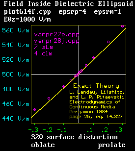
Figure 1(a). This is a test of the correctness of the calculation by numerically determining the electric field inside an ellipsoid of relative permittivity 4 when an external 1000 V/m field is applied parallel to the symmetry axis . For small eccentricities, this ellipsoid is approximately equivalent to a sphere of radius 1 being given a radial distortion of A S20(θ,φ) where A varies from -0.3 (oblate) to 0.3 (prolate). [Note: S20 = 0.630783 (1/2) (3 cos(θ)2-1) ]
The horizontal axis is A. The principal semi-axes of the ellipsoid are: a = 1 - (0.5) 0.630783 A, b = 1 - (0.5) 0.630783 A, c = 1 + 0.630783 A. In this case, coefficients of the permittivity c00 to c60 have been used. c80 and higher order terms are ignored. C++ programs used were: varpr27e.cpp (to calculate .clm file) and varpr28j.cpp (integrate to obtain potential). This figure was generated by plot614f.cpp. 52a.gif
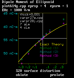
Figure 1(b). This is a test of the correctness of the calculation by numerically determining the dipole moment of the same dielectric ellipsoid. Method (1) is equation [10.18]. Method (2) is equation [11.10]. Method (3) is equation [12.5].
The yellow curve is equation [9.2], together with [9.3] and [9.7].
plot614g.cpp. 52b.gif

Other issues to address:
- Can this be generalized for the situattion where the permittivity is a tensor field εij(r) rather than a scalar field?

References:

L. D. Landau, E. M. Lifshitz and L. P. Pitaevskii "Electrodynamics of Continuous Media" 2nd edition Pergamon 1984 (volume 8 in Landau and Lifshitz Course of Theoretical Physics)
- See section 4 (pages 19-25) and sectioon 8 (pages 39-42)


Daniel Murray
Associate Professor
Math, Stats & Physics Unit
University of British Columbia - Okanagan
Kelowna, BC, Canada
daniel "dot" murray "at" ubc "dot" ca

For a list of related articles click here.


Hosted by www.Geocities.ws

1