Home Page First Cliff

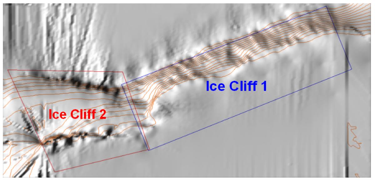
The second cliff, just to the west of the second cliff looked at a slightly different aspect and included some other features evident on the ice cliff. These comprise of ledge or step features and a large area of, what appears to be, 'blue ice'. For a comparison of the locations of the two cliffs and the difference in aspects see Figure 1 below.

Figure 1. A vertical view showing the relationship between the two scanned ice cliffs.

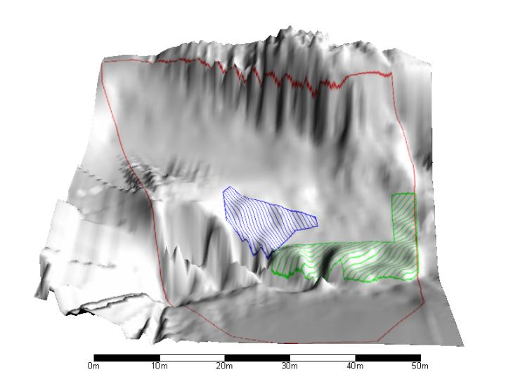
Initially the second cliff was scanned with a horizontal and vertical resolution of 1.0 metres. Using the default isotropic kriging interpolation algorithm, the surface shown in Figure 2 is produced from 1178 data points. There are, however, some visible anomalies in the data.

The second anomaly can be seen at the bottom of the cliff where a number of deep gullys and sharp ridges are evident. This is caused by an overhang. Most terrain modelling runs into problems when a single X-Y coordinate can have multiple Z values, (which is essentially what defines an overhang). This is a difficult problem to overcome. One attempt has been made to rotate the digital elevation model through 90º so that the cliff appears to be lying on its 'back'. This is achieved by swapping the Y and Z coordinates, so the plan coordinates are now X and Z. However, in order to register a 'rise' in Y with an overhang the Y coordinates must be made negative, (a decrease in Y corresponds with a 'bulge' on a south-facing cliff).

Figure 2. A front-on view of the second cliff showing the area scanned, (outlined in red), and two features scanned in greater detail; the ledges, (green) and the blue ice, (blue).

Figure 3. A front-on view of the blue ice feature on the second ice cliff.

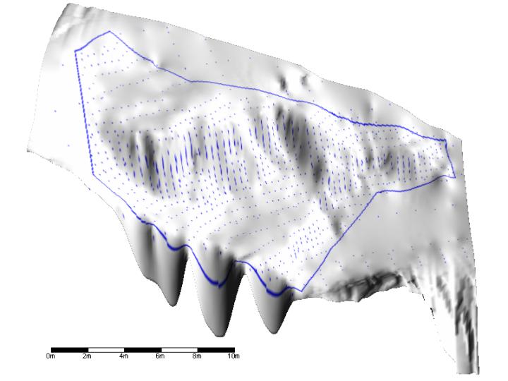
A second scan was made to examine a section of the ice cliff that had a smoother and 'bluer' appearance, indicated in blue in Figure 2. The hypothesis is that the response to ablation processes may be significantly different here to other sections of the cliff.

The scan was taken at a horizontal and vertical resolution of 0.25 metres giving 866 data points. The surface derived from these points can be seen in Figure 3 along with the distribution of data points from which the surface was obtained.

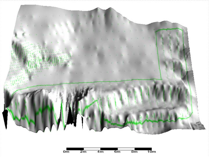
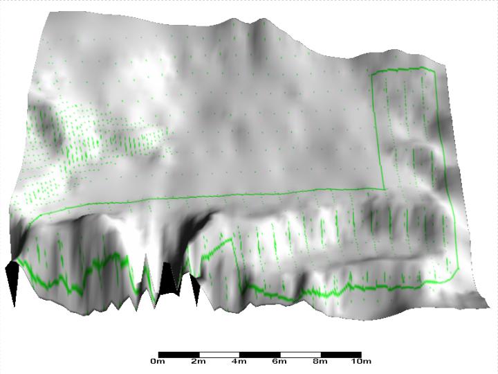
Finally a third scan was made to highlight a sequence of ledges or steps with a view to possibly separating out horizontal and vertical components of ablation or accretion. This scan was taken at a horizontal resolution of 1.0 metres and a vertical resolution of 0.1 metres. This was in attempt to highlight the change in elevation rather than change in the plane.

The cluster of points on the centre left are from the scan used to obtain the blue ice model and are not used in this analysis.

Figure 4. A front-on view of the step features on the second ice cliff with a grid resolution of 0.1 metres.

Further post-processing can improve the surface generated from this data. Firstly, it is thought that the resolution of the derived grid-based digital elevation model is too fine at 0.1 metres. This has been reduced to 0.3 metres in Figure 5, giving an overall smoother look to the surface. With a slightly coarser resolution the surface responds less to individual points as can be seen in the back wall of the model while still retaining the overall shape of the surface. There is obviously a trade-off between resolution and accuracy. Residuals calculated from the difference between the raw data elevation and the elevation from the model can be used as an indicator of accuracy, but inevitably some form of judgement must be used to obtain the optimum solution.

Figure 5. A front-on view of the step features on the second ice cliff with a grid resolution of 0.3 metres.

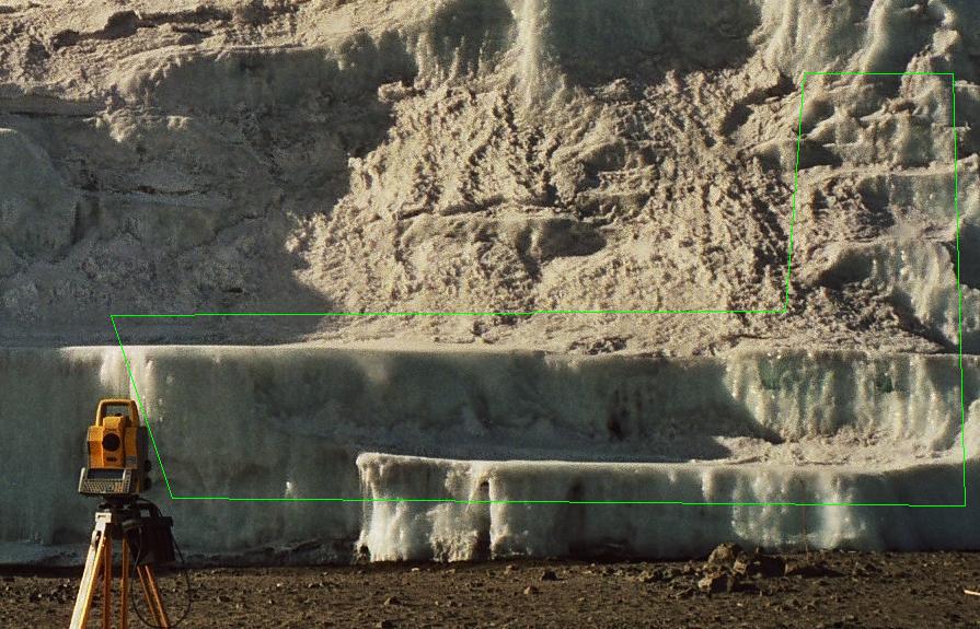
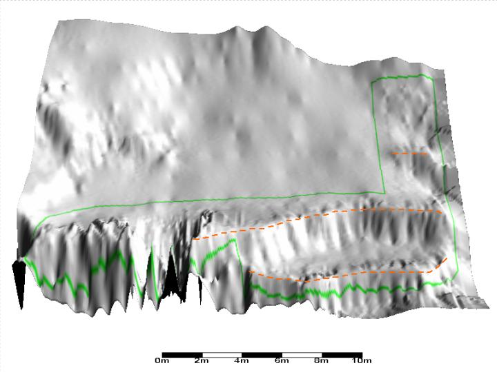
Secondly, on examination of Figure 4 it can be seen that the lip of the steps stand out at locations of observed data points. This gives a serrated appearance to the steps which does not conform to the real surface. As seen from the photograph in Figure 6 the edges are sharp and well-defined and some attempt should be made to replicate this form.

Figure 6. A photograph of the steps sequence on the second cliff showing, (approximately), the scanned area.

Figure 7. A front-on view of the step features on the second ice cliff with a grid resolution of 0.1 metres incorporating breaklines sen as brown dashed lines.