
Intended Learning Outcomes
At the end of this section students should be able to complete the following tasks.
- Describe the difference between hierarchical and partitioning clustering methods.
- Explain how changing the value of k is likely to impact on the cluster solution.
- List some of the potential problems with k-means clustering.
Background
The frequently used k-means clustering algorithm is both simple and efficient, as evidenced
by its description.
1. Decide on a value for k, the number of clusters.
2. Randomly separate (partition) the data into k clusters. The initial clusters could be
random or based on some 'seed' values.
3. Examine the clusters and re-partition the cases by assigning each case to its nearest
cluster centre. Usually a within-groups sum of squares criterion to minimise the within-
cluster variation, i.e. measure, and sum, the squared distances between each case and the
cluster's centre.
4. Recalculate the cluster centres as centroids.
5. Repeat steps three and four until an endpoint, such as number of cases moved, is reached.
Unfortunately a true optimum partitioning can only be found if all possible partitions are examined. Because this would take too long methods have been developed that should find a good, but not necessarily the best, partition.
The k-means algorithm is usually effective, particularly when the clusters are compact and well-separated, but it is less effective when clusters are nested. Estivill-Castro and Yang (2004) provide a detailed critique of the k-means algorithm and suggest alternatives based on medians rather than means. The main problems seem to be:
Because the algorithm typically begins with a random partitioning of the cases it is possible that repeat runs will produce different cluster solutions. If several repeat analyses are tried the 'best' will be the one with the smallest sum of the within-cluster variances. Alternatively bootstrapped samples could be used and the robustness of the cluster solution can be tested by examining how many times cases share the same cluster. Using the results from a hierarchical cluster analysis to place the cases into initial clusters appears to produce good results.
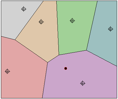
Unlike hierarchical clustering it is relatively easy to assign a new cases to the existing clusters. This is possible because the clustering partitions the variable space into Thiessen polygons or polygons whose boundaries are drawn perpendicular to the mid- point between two cluster centres. Any point falling within a Thiessen polygon should be assigned to that cluster (see figure below).
 |
Example analysis
This analysis uses data collected on 68 Hebridean islands (the location for much of my research). The data consist of the island's name, its location (latitude and longitude), the maximum altitude (m), area (km2), distance (km) to mainland Scotland, distance (km) to the nearest island, area (km2) of conifer plantation, the number of major rock types and the human population at the 1991 census. The data files (Excel format and Plain text) also have details of cluster membership from the five analyses described below.

In these analyses all of the variables, except for latitude and longitude, were used in five k-means cluster analyses. In all analyses the variables were standardised (because their measurement scales are very different) and five different values of k (2, 4, 6, 8 and 10) were tried.
Before examining one analysis in detail, the results from all five are summarised with respect to the total sum of squares. Recall that each cluster has a mean and the sum of squared distances, across all of the variables, can be found for each case within a cluster. Each cluster has a sum of squared distances for all of the cases in the cluster. If these sums of squares are summed a measure of the overall 'error' is obtained. If k is too small it is likely that dissimilar cases will be forced into the same cluster, producing a large cluster sum of squares. As the number of clusters increases this should decline as the cases in a cluster become inceasingly similar. However, there will come a point when the decline in the sum of squares is small relative to the increased difficulty in interpretation caused by the larger number of clusters. The figure below shows what happended to the total sum of squares (summed across all k clusters) as k increased from two to ten.
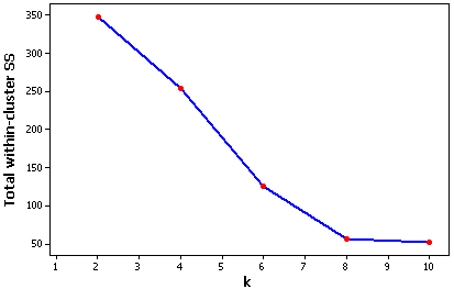
The total sum of squares declines rapidly from k=2 to k=8, there is only a very small decrease from k=8 to k=10. Consequently, with the aim of maximising parsimony, k=8 was preferred to k=10. The following details are for a k-means cluster analysis in which k=8.
Most clusters are small. Only two (4 and 6) are large. Unsurprisingly (since it is a sum) the within-cluster SS are larger for the largest clusters.
| Cluster | n | within | mean | maximum |
|---|---|---|---|---|
| 1 | 2 | 0.35 | 0.42 | 0.42 |
| 2 | 5 | 7.90 | 1.17 | 1.77 |
| 3 | 2 | 25.02 | 3.54 | 3.54 |
| 4 | 12 | 1.02 | 0.28 | 0.44 |
| 5 | 1 | 0.00 | 0.00 | 0.00 |
| 6 | 39 | 20.77 | 0.55 | 2.50 |
| 7 | 1 | 0.00 | 0.00 | 0.00 |
| 8 | 6 | 1.46 | 0.48 | 0.69 |
Since the variables are standardised a negative value for a cluster mean indicates that the cluster mean is below the overall mean (which is 0). For example, cluster 3 includes the large island of Mull, hence the large mean (4.52).
| Variable | 1 | 2 | 3 | 4 | 5 | 6 | 7 | 8 |
|---|---|---|---|---|---|---|---|---|
| MAXALT | -0.158 | -0.102 | -0.063 | -0.154 | 1.269 | -0.144 | 8.002 | -0.143 |
| AREA | -0.364 | 1.315 | 4.517 | -0.336 | -0.360 | -0.212 | -0.081 | -0.355 |
| DISTMAIN | 1.665 | 0.663 | -0.771 | 0.896 | -1.051 | -0.652 | -1.058 | 1.947 |
| NIDIST | 1.001 | -0.283 | -0.274 | -0.165 | 7.365 | -0.105 | 0.331 | -0.276 |
| CONIFER | -0.170 | -0.169 | 4.603 | -0.170 | 0.759 | -0.152 | 0.191 | -0.170 |
| GEOLTYPE | -0.286 | 0.047 | 0.594 | -0.240 | 7.774 | -0.146 | 1.474 | -0.255 |
| POPN1991 | -0.379 | 2.117 | 4.197 | -0.305 | -0.372 | -0.297 | -0.379 | -0.374 |
The next table shows that clusters 1 and 4 are similar (small distance), while cluster 3 and 5 are the most dissimilar.
| Cluster | 1 | 2 | 3 | 4 | 5 | 6 | 7 | 8 |
|---|---|---|---|---|---|---|---|---|
| 1 | * | 3.44 | 8.71 | 1.40 | 10.76 | 2.58 | 8.82 | 1.31 |
| 2 | 3.44 | * | 6.30 | 2.96 | 11.53 | 3.16 | 8.91 | 3.28 |
| 3 | 8.71 | 6.30 | * | 8.37 | 13.08 | 8.11 | 11.31 | 8.69 |
| 4 | 1.40 | 2.96 | 8.37 | * | 11.30 | 1.56 | 8.59 | 1.06 |
| 5 | 10.76 | 11.53 | 13.08 | 11.30 | * | 11.02 | 11.61 | 11.61 |
| 6 | 2.58 | 3.16 | 8.11 | 1.56 | 11.02 | * | 8.33 | 2.61 |
| 7 | 8.82 | 8.91 | 11.31 | 8.59 | 11.61 | 8.33 | * | 8.88 |
| 8 | 1.31 | 3.28 | 8.69 | 1.06 | 11.61 | 2.61 | 8.88 | * |
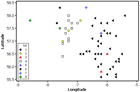
Although location variables were not used in the analysis it is obvious from the plot below that there is some spatial grouping in the clusters, albeit with some exceptions such as cluster 3 which has two members: Mull and Jura. These are both large, mountainous inner Hebridean islands. Cluster 2 is made up of large islands at the southern end of the outer Hebrides (Barra, Benbecula, Harris and South and North Uist). The large islands of Skye and Lewis are in their own clusters (Skye = 5 and Lewis = 7). Cluster 8 is made up of the more remote, uninhabited islands.
Related methods
The mean is just one of many averages and this is recognised in methods that use averages such as medians instead of the mean. The values for medians are less affected by outliers and could, therefore,produce a solution that is more robust. A more efficient algorithm replaces median by medoids. The PAM (Partition around Medoids) algorithm first finds k representative objects, called medoids and each cluster centre is constrained to be one of these observed data points. The PAM algorithm is more robust because it minimises a sum of dissimilarities instead of the squared Euclidean distances that are disproportionably affected by outliers. PAM is implemented in the free WinIDAMS software that can be ordered from UNESCO

Resources
Estivill-Castro, V. and Yang, J. 2004. Fast and Robust General Purpose Clustering Algorithms. Data Mining and Knowledge Discovery 8(2):127-150.