To develop an object tracking system that given the target’s attributes and a video clip, the system should able to identify the target in the video and track its movement. The application domain of object tracking includes surveillance, product examination in manufacturing line, and automatic guidance etc.

2. Literature Survey

The following are the resources available that explores the area of object tracking.

[1] has an implementation of a simple yet effective traffic monitor that can accurately measure the speed of a car travelling on highway. It involves the concept of background substraction and update as well as camera to real-world coordinate transformations.

[2] describes in details the how shape recognitions can be performed by histogram and signature recognitions.

[3] explains in details how a 2-pass segmentation algorithm is achieved.

The course series of [4] describes how background update should be done.

To refine the prediction model, Kalman filter could be used and [5] have details on the theory, applications and explanation of Kalman filter.

3. Problem Decomposition

Our object tracking system can be divided into four stages.

First Stage

The first stage is to identify the Region of Interest (RoI) by extracting pixels that are different from background and in the similar colour space with target. The goal of this stage is to limit the size of search space. The RoIs are represented by cluster of blobs.

Second Stage

In the second stage, we use segmentation method to convert the cluster of blobs into separate regions based on their connectivity. Small size regions are removed as noise and dilation is performed on significantly large regions to fill up small holes inside the blobs to enable the ease of further processing. We also obtain useful information from each of the region such as the bounding box, centroid, region size and also the horizontal and vertical projection. Hence by the end of this stage, our focus is reduced to a set of regions that are potentially our target.

Third Stage

With a set of potential regions, the third stage is to examine each one of them to determine their likeliness of being the target that we want to track. Each region is examined in three ways – histogram recognition, signature recognition and spatial locality evaluation. The first two are shape recognition methods and the last one is based on the assumption of the inertial properties of a physical object. These three methods will return three different scores.

The reason we use two shape recognition methods is that, we need each one of them to deal with different kinds of occlusion. Histogram recognition is good at recognizing object undergoing one sided occlusion but is not very stable to handle occlusion that is in the middle of the object. Whereas signature recognition can handle the latter type of occlusion nicely but fail to handle one sided occlusion due to the skewing of centroid position.

Fourth Stage

In the final stage, there is a heuristic to assess the object being examined to determine whether it is the true target. It is based on the scores obtained from the previous stage and the higher the score, the higher the chance that the object is the actual target. If the target is indeed found, then velocity prediction is carried out.

Fig 1. The problem decomposition of the object racking problem.

4. Scope of projects and Specifications

Scope

When developing our system we have assumed that comparable objects will appear in the same time with the target, and it is also possible that the target is not inside the video clip. Furthermore, the target object may undergo rotation, occlusion and size change (change of distance from camera). Our system should handle all these situations to determine whether the target is appearing in the video clip and if it is, which one is the target. The target are overlaid with red pixels and its trajectory of the last 20 frames is displayed

The system is required to work in real time, at a rate of 15 frames per second. Minor Lighting changes must also be catered for as well.

Specification

To acquire the target attributes a sample video clip of the steady target under different lighting conditions is used as an input into an attribute extraction application. The application will output a file containing the RGB space of the target, the signature and the histograms.

Our system runs on VirtualDub[6], where the inputs are the text file, our system (as a filter) and the testing video clip. The output is another video that shows the identified target, overlaid with red pixels if it does exist, and all potential targets identified are indicated by bounding boxes. The target also has a path that describes its movement over the last 20 frames. A file with scores is also created when the system runs, such that we could check the output of the heuristics of individual frames.

5. Design and Implementation

5.1 Background Subtraction

Background substraction is used as the first step to detect possible moving objects in the video sequence. This is only used to reduce the size of the search space by throwing out the background.

5.2 Colour Recognition

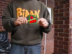
The RGB colour space of the target is first taken from a few video samples of the target under different lighting conditions. In our project we examine the objects in both under sunlight, shadows, indoor and outdoor environment. The maximum and minimum values of each colour channel observed in the sample are recorded and produced a rectangular prism which represents the colour space of interest.

Figs 1. Three images taken from a sample video sequence. The target object is the toy car model. The left image is taken under shadow. The middle image is taken with natural sunlight plus a close light source. The right image is taken with normal sunlight condition.

Since this step is used to eliminate the size of the search space and could eliminate the noise of flickering pixels in the background, therefore the colour space does not need to be very accurate and hence no learning algorithm or classifier are necessary as this approximation suffices the purpose. Another reason a rough approximation is preferred because a larger colour space would leave less holes in the segmented images in the later stage of processing.

5.3 Segmentation

After we form blobs representing the region of interest from colour recognition, we need to segment these blobs into different regions based on their connectivity of pixels. We use a segmentation algorithm called “two pass segmentation”. The advantage of this segmentation algorithm is it only passes through the whole image twice.

In the first pass, each pixel is assigned with a region ID by checking its down and left pixels (we passing image from down to up, left to right). These region ID need to be adjusted for the case of down pixel ID not equal to left pixel ID. So, the second pass is to adjust the region ID by checking the equivalency table. The diagram below briefly describe the process

Image with region IDs after first pass Region IDs after second pass

Equivalency table

After the two pass segmentation algorithm, region IDs are not continuous and there exists a lot of small segments due to noise. So, we need to pass through the image once more to normalize the region IDs and to remove segments which are smaller then a threshold of size in pixel. In our application, we remove any segment which is smaller than 200 pixels in size.

With a unique ID assigned to each of the pixels in the significant regions, we can form a bounding box for each region by finding the minimum and maximum values in both x and y directions. The centroid of each region can also be found by

X = (min X + max X)/2

Y = (min Y + max Y)/2

5.4 Merging segment

One disadvantage of our segmentation method is that, if our object is being occluded in the middle like the example in the diagram below:

We will have two segments represented by two region IDs for one object. That will be a disaster for shape recognition because the system does not even know these two segments belongs to one object, and will do shape recognition for each one of the two segments.

So we need to merge some of these segments that can potentially be a target. We brute forcedly check every two segments and merge them into one segment if they satisfy certain conditions (discussed below).

Merging of bounding boxes and finding new centroids are easy:

newMinX = min(minX₁, minX₂) newMaxX = max (maxX₁, maxX₂)

newMinY = min(minY₁, minY₂) newMaxY = max(minY₁, minY₂)

newCentroid X = (newMinX + newMaxX)/2

newCentroid Y = (newMinY + newMaxY)/2

And we have a merge table that works similar to an equivalency table to indicate which pair of segments is merged.

The merged segments are added at the end of the list of region as one more option for potential target. This means the system will examine region 0, region 1 and the region formed by region 0 and 1. Note that the condition for merging two segments cannot be too tight, because we don’t want to occlude any potential merge which may be a target. In our system, we merge every two pairs of segment which their centroids are closer than a threshold and the new formed centroid should be close to the target’s centroid in the last frame.

5.5 Dilation

Dilation is done straight after the segmentation to fill up any holes and jumps in the segmented regions, to increase the accuracy of the histogram recognition in the next stage. In our project a 3x3 mask is used.

5.6 Signatures

To obtain the signature of the target object, we use the distance from the centroid to the boundary of the object and follow this “radius” of the object for one revolution starting from the direction of the positive x-axis. We standardise the number of radii sampled to a fixed number 36, which means the sampling interval is 10 degrees. To allow fast recognition under different rotations, another 35 target signatures are generated from the initial one, each rotated 10 degrees from the previous one. This is a normalisation with respect to rotation.

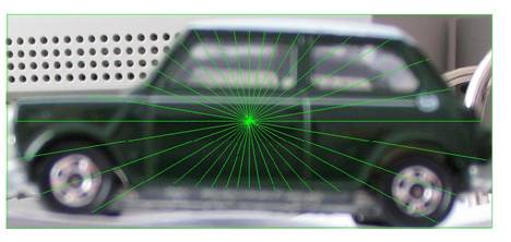
Fig 2. The signature of the target. It is a set of radii (indicated by the green lines) measured from the centroid to the boundary of the object. The sampling interval is 10 degrees generating 36 radii. Shorter sampling interval has higher accuracy yet incurs more processing time.

To recognise a potential object in a video once again we get its signature and compare them to the 36 differently oriented target signatures. The comparisons are done in division, that is each element in the object signature array is divided by the corresponding element in the target signature array, to obtain an array of ratios. Out of the 36 arrays the one that yields the lowest ratio variance then indicates a higher correlation between the true target and the object. Ratio is used as the measure of similarity because is invariant to the size of the object, unless it is so small that quantisation error becomes significant, for example, when the object is less than 30 pixels in size.

Toy Car

Triangle Cardboard

M&M

Pack of Tissue

Lowest Variance

0.0099

0.1351

0.0848

0.0542

Score = 1/std. dev.

10.05

2.72

3.43

4.30

Table 1 Comparison of the lowest variance between different objects against the toy car

This step is performed to all identified potential targets, and each of them has its own lowest variance which indicates the closest match in both the shape and rotation. A score is obtained by the inverse of the standard deviation (see Table 1). The score must also be above a certain threshold, in our project 4.00, such that it is not a false positive.

5.7 Histogram Recognition

Histogram Recognition uses the horizontal and vertical projection of the target object as a feature for object recognition. Unlike signature recognition, histogram cannot tell the exact shape of the object that it is recognizing. It can only determine the degree of similarity between two objects. However, histogram recognition is expected to have higher tolerance to size change (i.e. distance from camera change), rotation and also to some degree of occlusion.

5.7.1. Target Histogram Acquisition

In histogram recognition, the target shape is predefined as the shape histograms. We obtain histograms by projecting the target object in the rotation of 0, 45, 90, 135, 180, 225, 270 and 315 degrees. And for each degree of rotation, we have a horizontal projection as well as a vertical projection. So in total, there are 16 histograms for the target object. Also, the corresponding width and height of the bounding box (length of horizontal and vertical histogram) for each rotation is passed as an input.

The target object provided for histogram acquisition can be in arbitrary size (arbitrary distance from camera). However, as we want the shape histogram to be representative, we prefer to use a target which is rather close to the camera (larger in size).

5.7.2. Adjust Comparison

As object goes far away from camera, it becomes smaller in size and vice versa. For these cases, compare histograms columns by columns may not work because the smaller object will skewed from where we started to compare. Comparing the histograms from the middle to two sides seems solved some of the problem. However, it will make the columns of two sides become unrepresentative.

So, the way we comparing histograms is first to identify the object with smaller size in pixel. And then compare each column in the smaller object with the “representative” columns of the larger object. The diagram below is a simplified example for the problem.

Assume our predefined target object has histogram with length 200, which is larger then the object to be recognized that with length 5. We are going to choose 5 representative columns from the larger histogram to compare with each of the columns in the smaller one. Since each of the columns has to be equally space, the spaces between representative columns will be the larger length divided by the smaller length, that is, 200/5 = 40. This means we jump 40 columns every time when comparing with next column of the smaller object.

The reason I choose this high contrast in size is to show that the comparison is also subjected to skew effect. In this example, the space between the leftmost column and the first comparison is zero, where the space between the rightmost column and the last comparison is 40. To solve the skew effect, we have to share the space between leftmost and rightmost columns, which is, move all comparison by half of the jump space to the right. Instead of doing the first comparison on column 0, we now do the first comparison on column 20 (40/2 = 20), so that the last comparison will be on column 180.

5.7.3. Adjusting height

The size of an object directly related to the height of the columns for the histogram. So, we also need to adjust the height of the columns to adapt to size change when comparison. For example, if our predefined target is larger than the object to be recognized, we have to subtract each column from the target histogram by a factor before comparison or vice versa.

Assume we are comparing the histogram of two objects, one larger than the other. The larger object has size 600 pixels and 100 columns in histogram, where the smaller object has size 400 pixels and 80 columns in histogram. If H_i is the i^th column in larger object’s histogram and h_i is the i^th column in the smaller object’s histogram. The following will be their relation with size.

H₁ + H₂ + H₃ + … + H₁₀₀ = 600 pixels

h₁ + h₂ + h₃ + … + h₈₀ = 400 pixels

To adjust the histogram for the larger object, we assume that the 100 columns will equally shares the 200 pixels size different. Hence, we subtract every column of the larger object’s histogram by 2 (200 pixels divided by 100 columns).

Generally, the normalize factor to adjust column height is: (size different / number of columns of larger object). And for column by column comparison, we check if

[(H_i – normalize factor) – h_i] < Threshold

In our system, threshold of 5 is sufficient to recognize object. If the difference is smaller than the threshold, we count it as a “hit”. And the score will be the number of “hit” divided by number of comparison which is the number of columns of the smaller histogram.

5.7.4. Score Calculation

Output of histogram recognition is a score indicating the similarity of a region with the predefined target. As stated above, the score is the number of “hit” divided by number of comparison. But we want the score to be out of 100, so we time it by 100.

We obtain the average score from vertical and horizontal projection comparison for each of the 8 rotation target. And we choose the highest score among these 8 rotation score as our final score for that region. The idea is that, if the region is in fact the target object, the most similar rotation will output the highest score. On the other hand, if the region is in fact not the target object, we expect all of the 8 rotations will output similar score which is not high.

5.8 Spatial Locality

To identify the object of interest the spatial locality is taken into the account. The idea is that if a target appears in the current frame, it is very likely that in the next frame it will reappear in the current neighbourhood. Therefore an object identified as a potential target that is closer to the predicted position has a higher score in the heuristic that one which is further. The heuristic in assigning the score is inversely proportional to the error, that is the difference between the predicted position and the actual position.

Nonetheless in the current frame if the target is falsely identified, that is a false positive, then this assumption is going to let the error propagate into the next consecutive frames. As a result in the final heuristic the factor of the spatial locality is dynamically adjusted such that when it is less certain in the target visual recognition, we will trust less on this method.

Fig 3. A heuristic that is based on the spatial locality. The score is equal to the inverse of the error, which is the difference between the predicted and actual positions of the target at time k, so that the larger the error it is less likely to be the desired target object.

5.9 Final Heuristic

In the final step the scores from the object recognitions and spatial locality evaluations combine together. The final score is found from a weighted sum of all three components, however the weights are dynamically adjusted to reflect the current certainty.

Final Score = Histogram Weight * Histogram Score +

Signature Weight * Signature Score +

Locality Weight * Locality Score.

where all the weights sum up to one, and each individual score is capped at 100.

In particular, it is designed to tackle the fore-mentioned side-effect from the assumption of spatial locality that it can lead to a propagation of error if a false positive occurs in which case a high score is kept assigned to a falsely recognised object. As a result when both the histogram and signature recognitions both give low marks to an identified object, the weight of the locality evaluation is reduced to indicate that the uncertainty of the object. Thus even if the locality is misleading there is much less reliance on this evaluation.

Our system records all the scores over the last ten frames. The measure of certainty about the target visual feature is a direct count of how many times the shape recognitions scores are above some pre-defined minimum thresholds. From this we can derive the weight of the locality evaluation, which is:

Locality Weight = 1/3 * (certainty / 10).

Histogram Weight = (1-Locality Weight) / 2.

Signature Weight = (1-Locality Weight) / 2.

The result of such adjustment is satisfactory. Table 2 that shows its effectiveness.

Table 2. The result of spatial locality and dynamic heuristic weight adjustments

	Without Spatial Locality	Spatial Locality without Dynamic Weight	Spatial Locality with Dynamic Weight
True Positive	954	923	1039
True Negative	128	151	201
False Positive	103	146	8
False Negative	75	40	12
% true identifications	86%	85%	98%

5.10 Prediction of Next Position

The velocity prediction is performed when a target is successfully identified. The prediction is based on previous states of the target. From the velocity of the previous frames, the weighted sum of average of the actual velocities over the last five frames is the found. The error in the approximation is also used. Finally the predicted velocity for frame k+1 is derived as follows:

Fig 4. The weighted sum of average of actual velocities indicates the inertia of target. In our project, we consider the previous five values, and we assign more weights to more recent velocities (that is W_k > W_k-1 > … > W_k-i+1)

6. Testing and Result

In the testing stage, our system is tested with various situations that are carefully planned. Each of the situations testing an individual part of the system, and the results are obtained from output video or system printouts for evaluation.

When target not exist

The first test we have is to show an object that has same colour and comparable shape with the target and the real target is not shown, and see if it will falsely recognize the object as target.

Frame	153
Histogram (out of 100)	33.5
Signature (out of 100)	35.8
Spatial Locality(out of 100)	0
Total	34.7

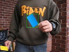
The result of this test is acceptable. Both of the histogram and signature recognition give low score to the shape. And the spatial locality output 0 because there is no object being identified. The bounding box and centroid formed means the system identified it is a blue object but it is not overlaid with red pixels means the system knows it is not a target.

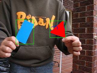
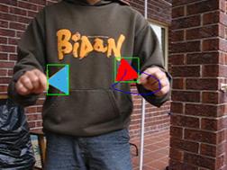
Recognize with comparable colour and shape

The next test is to see if the system can identify the target when there is another object with comparable colour and shape appears beside the target.

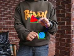
Frame	662
Region	Triangle
Histogram (out of 100)	85
Signature (out of 100)	88.4
Spatial Locality (out of 100)	98
Total	90.06

Frame	662
Region	Circle
Histogram (out of 100)	60.5
Signature (out of 100)	40
Spatial Locality (out of 100)	42.76
Total	47.75

Red overlaid pixels appear on triangle indicates that it can recognize the triangle as target, because both of the histogram, signature and spatial locality evaluation give high score to triangular region. Histogram recognition returns a relatively high score to the circular region. However, the low score in signature recognition and spatial locality even out the effect and so that the circle’s score is not too high.

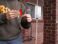
Rotation of target object

The target object is rotated to test if the shape recognition method can recognize object in different rotations. The target object is rotated from frame 553 to frame 589 clockwise.

The overlaid of red pixel doesn’t change and the score of both histogram and signature recognition give steady score about 80 to 90, indicating both histogram and signature recognition can adapt rotation well.

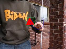
Distance Change

The target object and a comparable object is placed side by side and moved away and than towards the camera. This test is to see if our system can do recognition well in changing of size.

Frame	1223
Region	Triangle
Histogram (out of 100)	57.4
Signature (out of 100)	63.6
Spatial Locality (out of 100)	100
Total	73.67

Frame	1276
Region	Triangle
Histogram (out of 100)	74.8
Signature (out of 100)	95.2
Spatial Locality (out of 100)	100
Total	90

When the target object is far away from camera, the general score for shape recognition is low because there are less comparable features that can indicate its shape. However, the spatial locality still gives a high score due to its steady movement. As a result, the object is mostly recognized by its spatial locality.

When target is very close to camera, shape recognition gives a reasonable high score. This proved that our shape recognition is able to cope with size change.

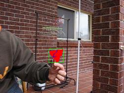
Undergoes Occlusion

There are two types of occlusion we tested, middle occlusion and one sided occlusion. Middle occlusion will separate target into two segments and merging of the two regions is needed. Whereas one sided occlusion will change the shape of bounding box and skewed the position of centroid.

Frame	1578
Region	Triangle
Histogram (out of 100)	56
Signature (out of 100)	74.2
Spatial Locality (out of 100)	98.8
Total	76.3

Frame	1812
Region	Triangle
Histogram (out of 100)	51
Signature (out of 100)	14.5
Spatial Locality (out of 100)	100
Total	55.1

For the middle occlusion, the two small bounding boxes are merged into one, and the new region is recognized as target. We can see that both shape recognition methods can handle this kind of occlusion and the spatial locality score helps scale the mark up.

For the one sided occlusion, signature recognition failed to recognize the target because the position of centroid has skewed. In this case, spatial locality plays an important role to track the target. But as the occlusion continues, the system started to trust less on the spatial locality. This is due to the low scores in shape recognition that make the system suspecting the current target is false.

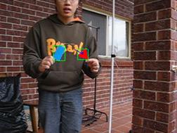
Two Blue Triangles

The final test is to test the effect of spatial locality, two identical targets (blue triangle) is placed in front of camera, one go into the camera’s view earlier then the other.

Frame	1934
Region	Triangle (Target)
Histogram (out of 100)	94.2
Signature (out of 100)	85.4
Spatial Locality (out of 100)	89.4
Total	89.67

Frame	1934
Region	Triangle
Histogram (out of 100)	92.6
Signature (out of 100)	90.1
Spatial Locality (out of 100)	44.3
Total	75.67

The first triangle is recognized as target, then the one that enters the view later is not recognized as target because of the spatial locality evaluation results in a low score for the second triangle.

7. Conclusion

In this report we have implemented an object tracking system that can track an object in real time video sequence. Our problem is essentially broken down into background substraction, colour recognition, segmentation, shape and object recognition and finally a prediction for the next state. The result was satisfactory and we have seen how a vision system tackles problems from a low level image processing to high level recognition and heuristics.

8. Future Improvements

8.1 Background Update

Background update can allow the background to change and adapts to lighting changes and fluctuations. In our project, we have implemented a background update that is efficient in architecture with the use of double buffering and amortised update. Yet the decisions of which pixel to update and how to update it are not straight forward. The problems we have encountered are:

How to choose an update strategy that will not treat flickering noise as new background pixel.
If the target object becomes stationary or moving too slow, we cannot absorb its image into a background.
Other objects that move inside the camera’s view but is not part of the background.

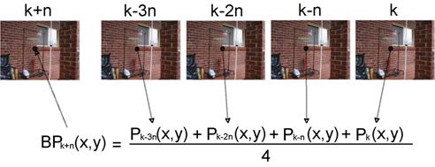
Fig 4. Background update. The update algorithm records a new image every n frames. The pixel mean is found and used in the new background for subtraction from frames (k+n) up to (k+2n-1).

Our approach in solving the first problem is to update the background from several images taken periodically over the last few seconds. From these images, we can compute the mean of all the pixels at (x, y) and form a new background pixel at position (x, y) (see Fig 4).

This method does not solve the other two problems though. To avoid updating the target whether it is stationary or not, the update can be performed after the recognition step such that the pixels belonging to the target are not considered in the update.

For other objects that sweep pass the camera, we can avoid update their pixels into the background by throwing out any “radical” pixels, because these objects will not stay in the same position in the image for a long period (otherwise they can be treated as the background). Hence when the mean pixel is calculated from the pixel set, the variance is also found. If any pixel from the data set falls outside, for instance, one standard deviation from the mean, they are not considered for update. Finally the new mean pixel is found from the remaining pixels and this becomes the new background pixel.

Due to time limitations nevertheless we have not carried out the implementation of the stages that solve problems 2 and 3. Hence the background update is not used.

8.2 Kalman Filter in Prediction

We can model the movement of the object in linear state space model with the state vector (P_k, V_k,)^T which represents the position and velocity of the target at time k. With the assumptions that the process and measurement noises are white and initial values of the state are Gaussian, Kalman filter can be used in the prediction to minimise the error.

9. Reference

[1] Speed Trap, C.D. Coro, http://www.cs.princeton.edu/~cdecoro/traffic/

[2] Digital Image Procession, R. Gonzalez and R. Woods, Addison Wesley, 2002.

Pattern Classi_cation, R. O. Duda, D. Stork, and P. Hart, John Wiley and Sons, 2000.

[3] Object Recognition, X.L. Zhuo http://www.sccs.swarthmore.edu/users/01/xianglan/e27/objRecognition.html

[4] Sensory-Motor Systems, Randal C. Nelson, http://www.cs.rochester.edu/users/faculty/nelson/courses/vision/vision.html

[5] Kalman Filtering , M.I. Ribeiro, http://omni.isr.ist.utl.pt/~mir/pub/Kalman-Filter.pdf June 2000.

[6] VirtualDub, Avery Lee, http://www.virtualdub.org 2004

[7] VirtualDub Filter SDK Tutorial, Avery Lee, http://www.virtualdub.org/filtersdk 2003